
Scratch 3D Project Development
By the 3D Graphics and Scratch Group.
This Book, created by 3D Graphics and Scratch (3DGaS), is intended as a comprehensive guide to modern 3d Scratch graphics programming. The book starts from simple concepts before branching to a variety of higher level concepts. Beginners are advised not to skip sections to avoid missing crucial foundational information.
For those with a general understanding of fundamental concepts like pre-calculus, geometry, optimization, and best practices, it is possible to jump directly to Rasterization and Triangles. The book also includes a Glossary for definitions of common vocabulary, a valuable resource for both novices and experienced programmers.
— The 3D Graphics And Scratch Group
Contribution Rules
- Never use generative AI in any form.
- No griefing.
- No harmful content.
- Ask people who wrote paragraphs before editing, moving or deleting their work.
- In case of accidental griefing, contact admins or the author to restore the damage.
- Don’t overwhelm with too many details your work, it needs to be balanced all over the book.
- Add your name to the credits.
Coding In Scratch
derpygamer2142, scratchtomv, BamBozzle
A deeper understanding of 3D graphics relies on an understanding of trigonometry and vectors. These appear in almost every algorithm in some form. Some chapters in this book will use more advanced mathematics for specific techniques, which will be explained when needed.
The Basics
World
derpygamer2142, scratchtomv, BamBozzle
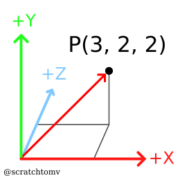
- A standard 3D coordinate system is (x, y, z).
- The coordinate system used throughout this guide looks as follows:
- The
originis the point in 3d space that has the coordinates (0,0,0).
Vectors
derpygamer2142, scratchtomv, BamBozzle
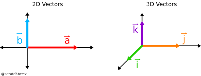
- A vector is a set of numbers similar to a coordinate. They usually describe a movement (called a translation) or direction in space. In 3D, vectors are most often found with 3 values, denoted as x, y and z.
- A vector has a length, or “magnitude”, that can be calculated thusly in 3D: √(x²+y²+z²)

-
A vector with a length of 1 is called a “unit vector”.
-
Dividing each component (x, y, and z) of a vector by the vector's length is called “normalizing”, and results in a unit vector pointing in the same direction.
Geometry
derpygamer2142, scratchtomv, BamBozzle, 26243AJ
- A point is similar to a vector, having a specific number of values, usually 2 or 3 when working in 3 dimensions. They are used to describe a position in space.
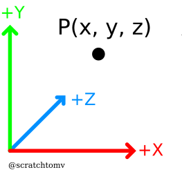
- A ray is a line in space which begins at an origin (a point), and extends infinitely in a particular direction (a vector).

- A plane is an infinite flat surface that extends across space. They can be defined in a number of ways, but most often by their normal (the direction the face of the plane is pointing) and their distance from the origin.
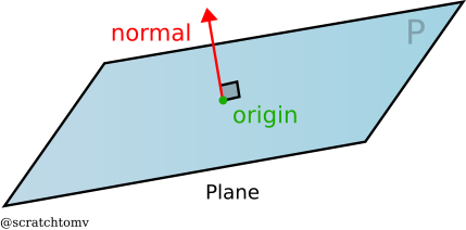
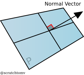
- A normal is a vector perpendicular to a surface. These are often normalized.
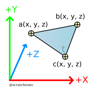
- A triangle is made up of 3 points, with the space between them filled in. Triangles are commonly used in 3d graphics because you can make any shape out of them.
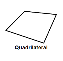
- A quadrilateral (commonly referred to as a quad) is made up of 4 points. Although not many scratch 3d engines directly support the rendering of quads (further elaborated upon in later chapters), they are often used in 3d models, making them an important aspect to consider when creating a 3d mesh / object loader.
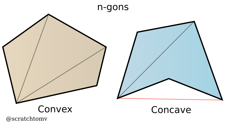
- An n-gon is a shape made up of an n number of points. In scratch these are almost never directly rendered, and are instead split up into many triangles within the object loader. (further elaborated upon in later chapters)
Trigonometry
scratchtomv, derpygamer2142
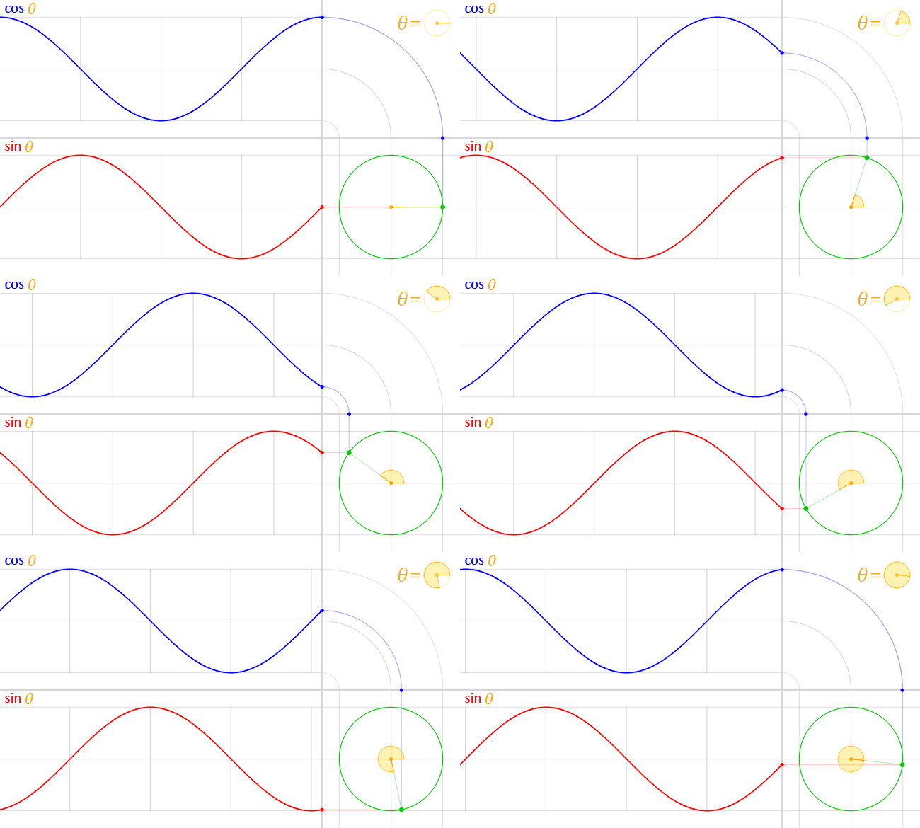
- Sine, cosine, and tangent(often shortened to sin, cos, and tan) and their functional inverses of arcsine, arccosine, and arctangent(asin, acos, atan) are trigonometric functions. They are used to describe the relationship between lengths, angles, and more. The specifics aren’t really relevant to 3d graphics very often, and are mostly used for rotation.
- Trigonometry functions can either use an input in degrees or radians. Radians are a form of describing rotation as a position on a circle with a radius of 1. One full rotation in radians is 2π.
Degrees work the same as radians, but they don’t need π to represent 1 full rotation, hence keeping the calculations simple. One full rotation in degrees is 360 degrees. - You can convert from radians to degrees by multiplying the radians by 180/π, and from degrees to radians by multiplying by π/180. Scratch uses the degrees system, and that is what we will use throughout this guide.
Matrices
badatcode123, derpygamer2142, scratchtomv, Krypto
A matrix is an array of numbers or expressions with rows and columns. Matrices are useful for many things, they make expressing rotations or transformations very easy.
Computations with them will be often simplified in Scratch as literal expressions, so you don’t need to really understand them to make 3D projects.
Matrices can be classified based on how many rows and columns they have, the matrix above is a 2x3 matrix because it contains 2 rows and 3 columns. We can multiply matrices with vectors. However, this isn’t commutative, so you need to be careful about in which order you do this.
An important matrix that is used throughout 3D graphics is the transformation matrix, it is a 4x4 matrix and can be used to convert between world space and a local space, it is often used to convert to camera space. To do this, multiply a vector (the vector being a vertex you are transforming in this case) with the transformation matrix.
In scratch, we usually use 3x3 matrices instead of a 4x4 matrix. We use a 3x3 matrix because it’s much easier to calculate its values, although a 4x4 matrix might make it faster and easier to scale and translate objects.
Matrix multiplication is performed by multiplying the corresponding rows and columns, then adding them together.
Here is an example in which the matrices and
are multiplied.
Rotation Matrix
26243AJ
A rotation matrix is a transformation matrix that is used to apply rotation on a column vector using the right-hand rule. However, due to the nature of matrix multiplication, the right hand rule is only valid when multiplying the matrix by the point and not vice versa.
The 2 dimensional form of this matrix has the following form:
Where θ is the degree you want to rotate the vector by. Using this, a point can be rotated around (0,0) by simply applying matrix multiplication.
Which can be simplified down to
Unlike in 2 dimensions, in the third dimension there are 3 basic rotations: rotation around the x axis, rotation around the y axis, and rotation around the z axis. Thus, there are 3 general rotation matrices for each individual rotation.
These can each be derived from the 2d rotation matrix, by rotating two out of the 3 axes.
For example, the rotation matrix for rotation around the x axis can be derived by keeping the x axis unchanged, and applying the 2d rotation matrix to the y and z axes.
These matrices are listed below:
These matrices can also be combined into one single rotation matrix which applies all 3 rotations at once.
Best practices when writing scratch code
scratchtomv
- Avoid using scratch comments.

- Find appropriate variable names.
- Avoid using temporary variables, it will create conflicts at some points although they can be useful for reducing the amount of variables.
- Use functions instead of spaghetti code (but don’t overuse).
- Use functions with “Run without screen refresh” when possible, instead of using turbo mode (except when the function has a very large loop).

- Don’t use clones for resource-intensive computation. In 3D programming we will almost never use them.
- Try to avoid most built-in scratch functions. You should really be working with variables, lists and operators exclusively.
- Use local variables when you can instead of global ones.

- Clean and organize your code. Be careful with the clean up blocks function, as it can move blocks to places which may not be ideal for some
- Don’t use one big sprite for all your code, it will slow down your project when in editor [i’m devastated - bozzle] [same - jfs22] [heartbraking - spog] [died of sad - derpy] [literally crying rn - spinning] [ain’t no way- AJ][lol - scratchtomv] [i refuse to accept this - 3TheHedgehogCoder3][I used to think broadcasts were slow, but I had to noooo - rinostar]
Running Scratch code
scratchtomv
3D projects run really slow on vanilla Scratch, as it uses a JavaScript interpreter to run the code block by block.
Fortunately a Scratch fork called TurboWarp allows projects to run blazingly fast by compiling them to JavaScript. It was created by GarboMuffin and is nowadays vastly used by the Scratch community.

turbowarp logo
Optimizing critical algorithms
Krypto
RTC Table :
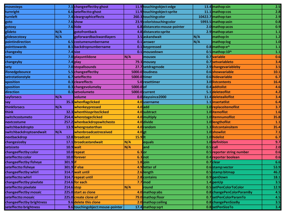 (RTC table by Chrome_Cat on Scratch)
Some of Scratch’s blocks are very slow and should be avoided the majority of the time.
The main blocks you should avoid are the list contains, item # of list blocks (both have a time complexity of O(n)) and touching blocks (Scratch needs to scan the entire stage). As you can see in the chart above, they have an rtc of above 35. Compared to addition blocks, they are at least 35 times slower. In most cases, in 3D you will usually not need to use these blocks.
If you do need to use these blocks (Searching for a name in a list, color scanners etc.) you can probably replace them with better alternatives or bake them at start.
Examples of blocks to avoid :
<touching color () ?>
(item # of [thing] in [Example List v])
<[Example List v] contains [thing] ?>
Complexity
26243AJ
Complexity is a measure of the performance of code when scaled up, and includes both memory and computational efficiency. It is most commonly expressed in Big O notation, which is a mathematical notation that expresses how an algorithm will scale based on the size of the input(s), n.
- For example, an algorithm that gets the first value in a list would be O(1), as even if the list had 20,000 values it would take the same amount of time to compute as a list with 1 value.
- An algorithm that would add up every value in a list would be O(n), since if the list had 100,000 values it would have to add up 100,000 values, and if the list had 2 values it would only have to add up 2 values.
| Most common forms of Big O notation n is the input, c is a positive constant | ||
|---|---|---|
| Notation | Name | Examples |
| O(1) | Constant | Finding the first value in a list |
| O(log(n)) | Logarithmic | Traversing a tree / a binary search |
| O(n) | Square root | Adding up all color values in the first column of a square image |
| O(n) | Linear | Adding up all values in a list |
| O(nlog(n)) | Loglinear, Linearithmic | Common sorting algorithms, such as quicksort and merge sort |
| O(n^2) | Quadratic | Naive collision algorithms, insertion sort |
| O(n^c) when c > 1 | Polynomial, Algebraic | [EXAMPLES NEEDED] |
| O(c^n) when c > 1 | Exponential | [EXAMPLES NEEDED] |
| O(n!) | Factorial | bogosort |
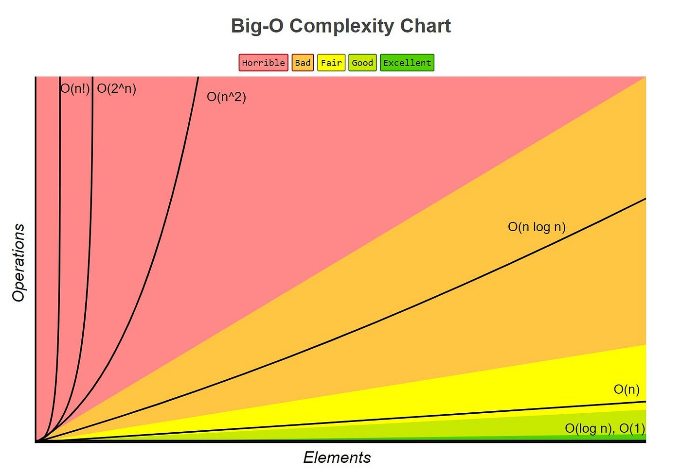
Important things to consider with Big O notation:
- Ignore Constant Multiplication; if a linear algorithm is twice as slow as another linear algorithm, it may be tempting to write it as O(2n). However, the big O represents all scaling factors, thus the 2 would be factored out and the expression would be written as O(n)
- Ignore less-significant terms; if an algorithm contains both O(n) and O(n^2) components, it may be tempting to write it as O(n^2 + n). However, big O notation only focuses on the fastest growing factors, which in this case would be n^2. Therefore, it would be written as O(n^2)
- A less-significant big O does not signify that an algorithm is better; Big O only shows a snapshot of how an algorithm scales, not how well it will perform in practice. At first glance, an algorithm that scales in O(log(n)) may seem better than an algorithm that scales in O(n), however, on small scale data sets the O(n) algorithm may perform better if it has a smaller O than the O(log(n)) algorithm. Although Big O notation can be very useful in providing a quick summary on how well an algorithm will perform, it should only be used as a rough guideline and it is still important to test the speeds of algorithms yourself.
Data Structures
In this chapter you'll learn how to store, import, export and use data efficiently.
Storing large amount of data in Scratch
scratchtomv
Lists are one of the only ways of storing large amounts of data in Scratch. They are pretty basic and only have a restricted set of operations that can be applied on them, some of them being very slow like “index of”. In large projects like 3D ones, they will often be thousands long, with the maximum being 200,000 items at runtime on Scratch.
Scratch stores lists in the project.json file contained in the .sb3 file. This project.json file has a 5MB size limit, which limits list size too.
Object representation in Scratch
scratchtomv
In Scratch, the basic way of storing data is by using variables, which can contain one information at a time. But how to store multiple pieces of information related to one object?
Let’s take the example of a dog : we need dog objects with multiple information related to it, like his name, his age, his race, his owner, etc.
Would look like this in C# :
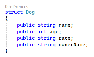
It can also be represented as a table :
| Data index | Property name |
|---|---|
| 1 | Name (string) |
| 2 | Age (int) |
| 3 | Race (string) |
| 4 | Owner Name (string) |
This object needs 4 data slots to be stored.
Storing objects in lists
scratchtomv
We just saw how to create one object, but what about handling thousands of theses ? Meshes can contain thousands of faces and vertices, we can’t hold all this data in a few variables, we need to use lists.
Lists in scratch are indexed by an integer starting from 1 (unlike most programming languages which start from zero), and each item in a list can hold values of any type Scratch variables can.
To store objects in a list, we need to partition it. There are multiple ways of partitioning a list, which we’ll see in the next parts.
Constant and defined object size
scratchtomv
If the objects stored in the list always take an n-amount of data slots, the list can be divided into groups of n-slots. It’s the most efficient and the most common way of storing objects.
| Index | Data | Object representation |
|---|---|---|
| 1 | Property A | Object 1 |
| 2 | Property B | |
| 3 | Property A | Object 2 |
| 4 | Property B | |
| 5 | Property A | Object 3 |
| 6 | Property B |
This simple scratch function create a dog (works for any kind of objects) :
define Add dog (name) (age) (race) (owner)
    add (name) to [my dogs v]
    add (age) to [my dogs v]
    add (race) to [my dogs v]
    add (owner) to [my dogs v]
…And is used like that
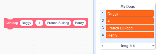
The object data can be accessed with two methods :
This is the fastest way, but you need to increment the dog index by 4 when looping through the list of dogs :
(item ((put your dog index here) + (put your data index here)) of [my dogs v])
This way is a bit slower and uses one more block, but is more straightforward :
(item (((put your dog index here) * (4)) + (put your data index here)) of [my dogs v])
This example accesses the age of the dog #0, and returns the second item for this dog, in this case 4 :
(item ((0) + (2)) of [my dogs v])
Constant but undefined object size using a list of pointers
scratchtomv
If the objects stored in the list can take any amount of data slots, the list can’t be divided into groups of constant n-slots. Thus, to be able to access its data correctly we need the use of another list containing pointers to the list containing the objects. This concept is used in a variety of situations.
| Index | Data | Object representation |
|---|---|---|
| 1 | Property A | Object 1 |
| 2 | Property B | |
| 3 | Property C | |
| 4 | Property A | Object 2 |
| 5 | Property A | Object 3 |
| 6 | Property B |
| Index | Data |
|---|---|
| 1 | 1 => (Pointer to object 1) |
| 2 | 4 => (Pointer to object 2) |
| 3 | 5 => (Pointer to object 3) |
Dynamic object size
scratchtomv
Dynamic object allocating is really slow and you should avoid it by using other storing methods, such as pre-allocating enough data slots.
But if you really need to be able to grow or shrink an object size, you can achieve it by using linked lists :
- When an object A needs to grow in size, use the “insert” block to insert a new data slot, then loop through all the pointer’s list and increase by 1 all pointers higher than the object A index.1
- When an object B needs to shrink in size, do the same as the growing operation but with the “remove at” block to remove the desired data slot, and decrease by 1 the pointers.
Mesh data in scratch
Storing
scratchtomv, krypto
The way of storing triangles is heavily defined by how it is used. One method is storing all triangles and all the vertices in two lists. The mesh data can be easily accessed by looping through these lists.
This is the easiest way to store your mesh data, new fields can be added according the renderer needs :
| Quads | |
|---|---|
| 1 | Vertex 1 index |
| 2 | Vertex 2 index |
| 3 | Vertex 3 index |
| 4 | Vertex 4 index |
| 5 | Material index |
| Vertex | |
|---|---|
| 1 | X |
| 2 | Y |
| 3 | Z |
| Ngons | |
|---|---|
| 1 | Vertex Start Index |
| 2 | Polygon Vertex Length |
| 3 | Material index |
| Triangle | |
|---|---|
| 1 | Vertex 1 index |
| 2 | Vertex 2 index |
| 3 | Vertex 3 index |
| 4 | Material index |
If you want to create a 3D project you can now jump right in the Rasterization and Triangles chapter.
Importing
scratchtomv
Importing an OBJ file is the easiest and most efficient way to import a mesh in Scratch.
Why use OBJ Files?
- They are fairly easy to parse since they are stored in the ASCII layout.
- OBJ is a file format, also known as wavefront, and is a very easy way to import a model from a 3D modeling program, to Scratch.
There are two main ways of importing an .obj file in Scratch : it can either be imported into a list, or pasted in a variable / input field. There are no “good” ways of doing it, but here we will approach the paste method.
The first step is to obtain an .obj file : it can be found online, or exported from Blender.
Once done, we can use a simple algorithm to decode the OBJ data, by reading it step-by-step.
- Skips the metadata at the beginning (#)
- (Optional) Reads the material name and links the material data to the following object. (mtllib)
- (Optional)Reads the object name (o)
- Reads all the vertices position data (v)
- (Optional)Reads all the uv data (vt)1
- (Optional)Reads all the vertex normal data (vn)2
- Reads all the face data (f)
In order to read this data, this function uses another function that reads and stores the characters until it finds a special letter combination such as “v”, and returns this data.
Full OBJ file specifications :
http://www.hodge.net.au/sam/blog/wp-content/uploads/obj_format.txt
If the .obj file includes UV data.
If the .obj file includes vertex normal data.
Texture storing
scratchtomv
There are two main ways of using textures in 3D projects :
| Method | Store all the pixel colors in a list used for all textures | Use an STTF (Stamped Textured Triangle Fill) |
|---|---|---|
| + | Allows for much more flexibility and color management later on. Can be projected perfectly. | Easy to import textures Doesn’t take place in the JSON Fast texture rendering. |
| - | Takes a lot of space in JSON (Can be bypassed by storing the data in image costumes) Takes a lot of time to render textures. | Texture projection isn’t accurate. It uses GB of RAM to render. |
| When to use ? | Projects that need : A lot of different textures, perfect projection, perfect sorting, not much FPS Fragment, shaders | Projects that need : More FPS, few textures |
| Example |
Using a list
scratchtomv
Using a list to represent a texture is actually representing a 2D texture as an 1D array of colors. These colors need to be in a Scratch-compatible format. If you’re not aware of color representations in Scratch, see Handling colors in Scratch.
These tools can be used to convert an 2D texture to an array of colors :
- Hex conversion :
https://xeltalliv.github.io/ScratchTools/Img2list/#hc1 - Decimal conversion : https://xeltalliv.github.io/ScratchTools/Img2list/#dc1
These textures can be rendered in 3D with a Textured Tri Fill, with or without a depth buffer. For more information look into Drawing Triangles.
If the texture list is taking too much place in the project.json file, it can be compressed or stored in a costume.
One common method is to compress the textures using tools like this one made by awesome-llama : https://github.com/awesome-llama/TextImage, and use an image scanner to read the sprite’s costume data like this one made by Geotale : https://scratch.mit.edu/projects/643721525.
Using costumes
scratchtomv
Since the equations involved in projecting costumes to 3D are complex, Chrome_Cat’s STTF 2 is often used: https://scratch.mit.edu/projects/888667870/.
How it is used :
- The texture is converted with this tool made by Chrome_Cat :
https://joeclinton1.github.io/texture-converter-js/ - The costumes are imported in the renderer sprite.
- They are rendered using STTF, see Drawing Triangles > Stamped
Rasterization and Triangles
BamBozzle
A rasterizer is a 3D engine which draws objects to the screen by filling in shapes. For example a rasterizer takes in a 3D model constructed from triangles and then draws those triangles to the screen to display the model. Confusingly, in the context of Scratch, “Rasterization” can refer to both the act of filling shapes to draw objects, and also to the specific technique of using a triangle filler that draws pixel-by-pixel (typically with a depth buffer). From here on, “Rasterization” refers to the former.
The first subchapter Drawing Triangles will teach you the theory about different methods of rendering a 3D scene in Scratch. Then Rendering Basics will teach you how to build the basis of a 3D raster renderer. Finally, Painter’s algorithm, BSP sorting and Depth Buffers will teach you about the different sorting techniques.
Drawing Triangles
BamBozzle
Every form of rendering discussed in this chapter exclusively1 uses triangles to construct the objects drawn on screen. This is for a few reasons. The first is that in order to fill an area in space, 3 or more points are necessary. A point or a line cannot fill an area in space, and so are not useful for representing surfaces.
The second is that triangles are necessarily coplanar, which means that for any 3D triangle, there always exists a flat plane that all the vertices can lie on. Due to how projection works, this means that a 3D triangle will always still look like a triangle when drawn to the screen, a property not held by any other 3D shape with more than 3 points. This greatly simplifies the process of rendering, as it is not necessary to determine what type of shape is being drawn, as it will always be a triangle.
The third reason is that there is one true way to draw a triangle. For 4 or more points drawn to the screen, there is not one “correct” way to fill the space between them, unless the points have a specific order, which creates its own problems.

Since shapes with fewer than 3 points are unsuitable, and shapes with more than 3 points come with a lot of inconvenience and vagueness attached, triangles are left as the most useful shape for representing 3D objects. As such, many triangle filling algorithms have been created on Scratch. The predominant methods are Incircle Filling, Stamped and Scanline.
Incircle Filling
BamBozzle
Incircle Filling is the most commonly used technique on Scratch as it is fast and flexible. It works by finding the incircle of the triangle, which is a circle which is tangent to all 3 of the triangles edges. This is the largest circle you can fit inside the triangle, and therefore drawing it with a single pen dot fills in the largest possible area. After this, lines are drawn along the edges to fill in the remaining area.
Since this method uses pen, it can fill in any triangle without visual bugs, and can also be set to fill in any color. Since it is a popular technique there exist many highly refined versions of it on Scratch. The 3DGaS group recommends the usage of Azex 3D, a highly-refined triangle filler created by tsf70 and kryptoscratcher.
There are some downsides to this technique. Since there is overlap of the lines used to fill the area, transparency is quite ineffective with this filler. At lower resolutions, depending on the filler used, some areas in the corners of triangles may not be filled, or the triangle may “spill over” into the surrounding area.
Azex (left) vs -Rex- (right) :
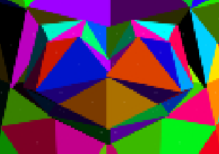
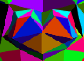
Scanline
BamBozzle
Another technique is to fill successive rows of pixels inside the triangle, known as “scanlines”. These rows do not overlap, and so transparency is quite a bit more effective using this method2. A high number of scanlines are needed to avoid jagged or imprecise edges. This has a large performance impact, so it is recommended to only use this technique for transparent triangles, or other necessary contexts, and not for general triangle filling. Modifying this technique allows for texture support, as well as Z-Buffer support.
Stamped
BamBozzle
It is possible to fill triangles using a stamped sprite. This technique can be very fast, as it prints the triangle all in one go. This technique also allows for free affine texture mapping by making the stamping costume textured.
Rudimentary versions of this technique split the triangle to be filled into two right angled triangles, and then select a costume of a similar right angled triangle for each. After correctly scaling and rotating, these two triangles are stamped to fill the specified region. This method leaves a visible seam in the triangle, has precision issues due to the discrete number of triangle costumes available, and has issues with texture mapping due to the split in the filled triangle.
Scratcher Chrome_Cat realized.
Some advanced Scratch 3D engines have limited quad support, on top of triangle support. This is done for small performance gains and in most cases is not worth the extra complication. The quads that these engines can render are also typically limited to being near-coplanar and convex, for the reasons discussed.
Due to Scratch anti-aliasing there may be very thin lines still visible using this technique at some resolutions.
Rendering Basics
BamBozzle
This section will walk through the process of rendering a 3D triangle, given its point in 3D space. This step is broadly the same regardless of the method of rasterization you are using, though there may be slight differences from engine to engine1
Projection
Reference: https://youtu.be/tX_x4iYvspU?t=128
Firstly, we must define a list of triangles. All models are composed of many interlocking triangles in a space, called model space. Each triangle also consists of three vertices. The way the triangles are defined by these sets of vertices is by using a list of indices that point to which vertex it will use.
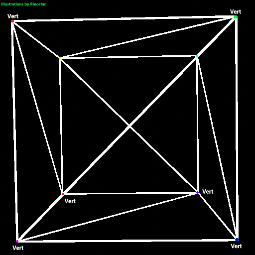
Here, I’ve shown what a cube would look like if we just rendered each edge of the triangle. I’ve also made colored dots, and text around them showing where each vertex is. As you can see, a cube has 8 vertices, and 6 faces. But, since this is composed of triangles, the cube has 12 tris2. If we were to just have each triangle have its own set of vertices, the renderer would have to do extra calculations to project the same vertices if these triangles were connected. That’s why indices are used. Here’s an example of this cube being represented in a mesh file:


As you can see, each vertex has a 3d point in space. This is usually represented as either coordinates, or vectors. Of course, all coordinates can be vectors, but not all vectors can be coordinates.
Above you can see the list of face data as well.
This entire code for just the cube model is pretty long, especially when you try to stuff vertex colors, uv data, and more inside each model, but that’s how it works. You can plainly see that each face has 4 numbers. The first 3 are pointers3, or indices to the vertices of the mesh, and the fourth one is just what color the face is. We won’t be covering face color yet. When getting model data, it’s generally a good idea to have your indices and vertices in separate lists during runtime. The reason I stored the mesh data like this is simply because of being able to more easily import meshes before running the engine. Plus, the mesh data just gets split into vertices and indices whenever needed. But what do we do with all this data?
Well, if you're just making a mesh loader or something similar, you can just skip these steps, but if you want a more advanced rendering engine (which can be turned into a game engine later), this step is nearly essential: we will need to project these meshes into world space. The reason for this is to be able to not only have multiple meshes rendering at once, but to also be able to freely move, rotate, and scale them at will.
Converting to World Space
So how do we do that? Well, with some vector math, of course! Expressing the scale matrix, which allows you to be able to stretch or squeeze objects in any axis, it looks like this:
.
Going back to the cube example, if we applied the scaling matrix, with S = [2 1 1], then the cube will turn into a rectangular prism:
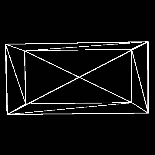
Next, the translation (or the moving thingy around) matrix. This is very weird, but here it is:
.
This matrix makes use of homogeneous matrices. I won’t go into detail here,4 but this just lets us have 4x4 matrices in 3d space. This will make translation possible, though. Next up, the rotation matrix. There’s already a page for that explained here: rotation matrix page in the book (pg. 13), so I don’t actually have to show it here. There’s also more talk about it later on, too. So now we know how to project the vertices to world space using math, but how do we implement it into scratch? Well, first we’ll have three variables, x, y, and z. This’ll be the variables that get transformed through each matrix. Note that the rotation will be in three axes in this case.
Each matrix is its own function, so here’s the scaling function:
It’s very simple, it just multiplies each component with the corresponding scaling component. Next up, the rotation triples!
They all look similar, except which variables are affected, and which components it uses.
Very simple, just a bit of trigonometry, though.
And finally, the translation function!
Also very simple, just like the scaling matrix, except you add the vectors together. And with that, you can position any 3d mesh into world space. Note that when trying to put multiple meshes into the world, you have to store the current length of the world vertices list (if all three components are stored in that one list, and you usually either skip indices to get each vertex, or you multiply the index, just make sure to divide the length by the number of components, which in 3d is 3) as a variable like Lv, and when you copy over the new indices, just add the indices with Lv, so as not to create something I like to call, face interference:
offset off:
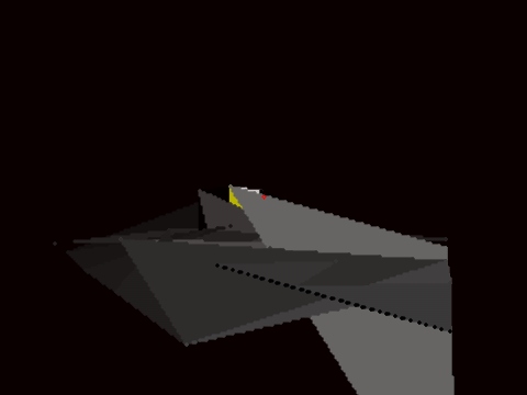
offset on:
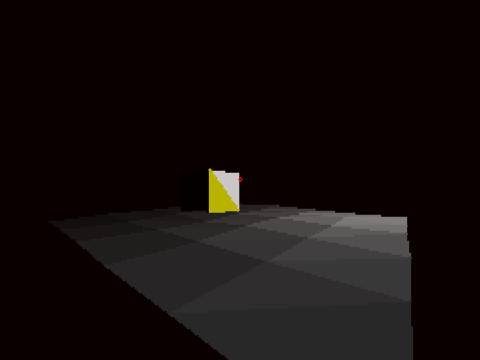
(In this case, offset is the variable to add with the indices for the mesh)
Next up, converting the entire scene in world space to view space.
Converting to View Space
Z clipping
Filling
Rendering n-gons
Krypto
One way to raster a polygon is with the fan triangulation. The way this works is that you “pin” one of the vertices of the polygon and then you go around the polygon creating triangles with the vertices of the pin and the current one you are looping around. As you can see in the image below, this triangulates the polygon. Furthermore, you can use quads in a painters engine to triangulate this polygon, adding a bigger performance boost when rastering polygons. This method of triangulation only works with convex polygons, however.
Some engines choose to perform the projection step before the sorting step when using painter’s algorithm.
tris will be short for triangles.
In c, or c++, you already know what I might be talking about.
Painter’s algorithm
SpinningCube
Painter’s algorithm is used by a large portion of filled-surface 3D renderers on Scratch. The algorithm’s name alludes to a technique a painter might use to capture a scene. The painter paints the objects in the scene from back to front, starting with the most distant object they can see. Since each new brush stroke may cover up brush strokes already applied to the canvas, the objects painted last appear at the very front, not obstructed by anything, while objects further back have been partially covered by objects in front of them. This ensures that surfaces that are behind other surfaces can’t be seen in the painting, as we would expect.
The algorithm involves the following steps:
- Sort polygons by depth
- Using the sorted list, draw each polygon to the screen in back-to-front order
Limitations
By its very nature, painter’s algorithm can never be fully accurate in all cases—there are always cases where it fails to correctly draw a scene, such as when there is no clear ordering of “back-to-front”:
Of these three faces, none can be considered the frontmost or the backmost. Intersecting faces pose a similar problem. Thus, painter’s algorithm is prone to visual artifacts. Even with simple objects it can often fail to correctly resolve the scene.
There are some ways to mitigate these artifacts. Backface culling can help remove some of the unnecessary faces from being sorted (This would fix the cube in the above example). How each face’s depth is determined can be altered to achieve different effects. Usually, the average of the Z depths of the face’s vertices is used, but this can be changed to use only the depth of the closest or furthest vertex, for example. Another strategy is to add an artistically chosen bias value to the determined depth based on certain expectations. A common problem is for smaller objects to be incorrectly sorted behind the geometry of the ground they rest upon. These objects could be slightly biased towards the camera to reduce the chance of this happening.
These strategies can be used to reduce the prevalence of visual artifacts in scenes, but there is no simple solution that can completely get rid of them. For perfect sorting, you need a more robust technique.
Binary Space Partitioning (BSP)
See dedicated article by littlebunny06.
Depth Buffers
urlocalcreator
In rendering using the scanline technique, using a depth buffer may be preferred rather than sorting triangles one by one. Using a depth buffer is fast, but at the consequence of forcing the scanline technique rather than a faster incircle filler.
In a situation in which you need a Z buffer, you can simply go along with the scanline technique and interpolate between the Z value for the edges of which you are rendering, then for every pixel, you save the Z value in a list if the Z value for that pixel is less than the one saved for the pixel from the previous triangles. It allows for you to have objects clip into each other as a benefit, and reduces strain on the CPU from sorting. There is no real consequence to having a Z buffer unless you want to use a faster rendering approach.
2 Images from the same engine but different rendering techniques
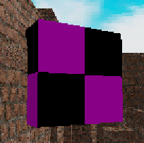
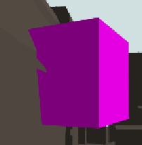
As you can see, rendering with a depth buffer can get rid of the triangles that should not be seen.
Another way you can see the depth buffer is in a shaded gray image. It resembles how far something is from the camera in the Z direction and can be called a depth map. A depth map allows you to do some cool shading effects later on in local space (which may be discussed in a later chapter).
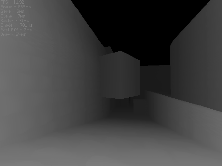
Ray-based 3D rendering
26243AJ, BamBozzle, badatcode123
Ray-based rendering algorithms use rays to render scenes. They work by shooting a ray(s) into the scene for each pixel, these algorithms are able to calculate the color and depth of these pixels. Many techniques for this exist, such as raytracing, raymarching, DDA, etc. The main difference between these methods is how they determine a ray intersects an object in the scene.
Ray-based rendering has the advantage of making it trivial to implement features such as shadows, reflection and refractions, which are usually much harder to do in other methods of rendering, such as rasterization. The drawback being that ray-based rendering is almost always slower than traditional rasterized rendering.
Basics
26243AJ, badatcode123
Mathematically, a ray is defined by an origin (a position in space) and a direction at which it travels. It extends infinitely from its origin in its direction, as seen above.
Although there are various methods to render a scene using these rays, the majority of them require each pixel of the screen rendered separately in a grid-like fashion. This can be done by iterating through the screen with 2 simple loops;
[Insert blocks here]
*In this format, resolution is defined by the size of each individual pixel. A resolution of 1 would produce an image with the same resolution as the vanilla scratch canvas.
**The pen size is scaled by 1.4, or the square root of 2, as circular pen dots with the same diameter as the height/width of the pixels would not fully fill each pixel.
***It is not recommended for these main render scene blocks to “run without screen refresh,” as these renderings can take up to several seconds to finish, which can cause the page to freeze or even crash if “run without screen refresh” is turned on.
For each pixel, a ray is created based on the position of the pixel and the position and rotation of the camera. The position of the pixel on the screen can simply be treated as the ray’s x and y direction, and the z direction is defined by the focal length.
[insert generic diagram of ray tracing here to elaborate on this]
Then the ray’s direction is normalized, as further calculations may require a normalized direction, and is then rotated relative to the camera.
[Insert blocks here]
The cast ray function shoots the ray into the scene, the specifics of how it does this is dependent on the method you are using, but it always finds the closest intersection point to the ray, as seen below.
[Insert diagram here]
As has been said already, the main difference between the methods are in how they find the intersection points.
define render screen (res)
    pen up
    set pen size to ((2) * (res))
    go to x: (-240) y: (-180)
    repeat ((360) / (res))
        set x to (-240)
        pen down
        repeat ((480) / (res))
            get pixel color (x position) (y position) :: custom
            change x by (res)
        end
        pen up
        change y by (res)
    end
For each pixel we need to perform a function to do ray collisions, but first we need to define the ray origin and ray direction. The ray origin for this case is the camera position, and the ray direction is defined as
define get pixel color (x) (y)
    set [ray origin x v] to (0)
    set [ray origin y v] to (0)
    set [ray origin z v] to (0)
    set [length v] to ([sqrt v] of ((((x) * (x)) + ((x) * (x))) + ((focal length) * (focal length)))
    set [ray dir x v] to ((x) / (length))
    set [ray dir y v] to ((y) / (length))
    set [ray dir z v] to ((focal length) / (length))
The focal length is how far the lens of the camera is from the aperture, this is inversely proportional to FOV and should be around 300. With the ray origin and direction defined, we can now use the ray algorithms to move the rays.
2.5D Ray-casting
2.5D raycasting is a unique form of 3D rendering. Instead of projecting polygons or casting rays for every pixel of the screen, in raycasting, we cast a single ray for every column of the screen.
This leads to significant performance improvements over raytracing, but it also places restrictions on the camera and world design. In a raycasting engine, cameras can only look left and right (although pitch can be faked by panning), and generally surfaces must be exactly vertical or horizontal (but as we’ll learn, there are clever tricks to get around this too.)
So why would someone want to create a raycasting engine? There are a few motivations. Firstly, raycasting is fast—a bare-bones, cuboid grid, shading-free raycasting engine can run at 15–30 fps in 480x360 in vanilla Scratch. Secondly, raycasting is simple—both conceptually and programmatically. This is why simple sprite-based raycasting is a popular project for 3D beginners, and plenty of tutorials for that can be found on YouTube, the Scratch Wiki, and on Scratch itself.
But although I’ll start with a simple conceptual model, I want to show you how raycasting can be pushed to its limits to create visually stunning, complex worlds with polygonal walls and ceilings, advanced lighting, and even terrain. Not many raycasting engines have done these things before—so buckle up for the ride!
“Raycasting?”
What do I mean by “raycasting” exactly? It’s just as the name implies—we’re casting rays in a virtual 3D world, then drawing the results on the screen.
Let’s start with a simple example. Let’s say we have a simple rectangular map, with outer walls, and a pillar in the center, like this:
████████████████
██            ██
██            ██
██     ██     ██
██            ██
██  @         ██
██            ██
████████████████
The camera is represented by the @ symbol here. Intuitively, we know that the camera can only see things which it can hit using rays. A person can only see something if there’s an uninterrupted line from their eye to the object. We also know that things appear smaller the further away they are. Can we use these facts to our advantage?
If we know the height of an object, and how far away it is, we can calculate its apparent height using this calculation: height / distance.
Floorcasting
Terrain
Sprites
Lighting
Shadows
Ray-tracing
26243AJ, badatcode123
Raytracing is a method of 3D rendering that uses ray-surface intersection functions to find the nearest intersection distance to an object, “t”, if the ray hits the object. A simple ray-surface intersection is the ray-sphere intersection, shown below.
define Ray-sphere intersection|sphere pos (x) (y) (z) radius (rad) color (r) (g) (b)
    set [nx v] to ((ray origin x) - (x))
    set [ny v] to ((ray origin y) - (y))
    set [nz v] to ((ray origin z) - (z))
    set [b v] to ((((ray dir x) * (nx)) + ((ray dir y) * (ny))) + ((ray dir z) * (nz)))
    set [c v] to (((((nx) * (nx)) + ((ny) * (ny))) + ((nz) * (nz))) - ((rad) * (rad)))
    set [t v] to ((b) * (b) - (c))
    if <((t) > (0))> then
        set [t v] to (((0) - (b)) - ([sqrt v] of (t)))
        check if intersecting (t) object color (r) (g) (b) :: custom
    end
define check if intersecting (t) object color (r) (g) (b)
    if <<(t) > (0)> and <(t) < (ray t)>> then
        set [ray t v] to (t)
        set [object color R v] to (r)
        set [object color G v] to (g)
        set [object color B v] to (b)
    end
Now we can test intersections with every object in the scene and then color that pixel the color of the object (reminder that the color of the object is from 0-1 not 0-255) that has the smallest t value or the background color if there are no intersections. Do the ray-sphere intersection right after defining the ray origin and direction.
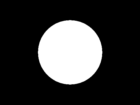
Expected output (circle radius of 25 and positioned at 0,0,100)
Ray-marching
badatcode123, derpygamer2142, jfs22
Raymarching is a method of ray-based 3D rendering that steps rays through a scene in order to approximate collisions. Raymarching is unique however, in that it uses Signed Distance Functions, or SDFs, to step by the most it can without hitting an object in any direction. When inside an object, SDFs return negative, hence the signed part of the name.
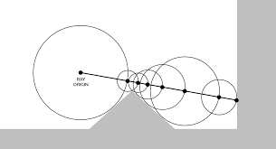
A ray is considered to be intersecting an object when the SDF is less than some arbitrarily small threshold, often called “epsilon”. Additionally, to stop infinite steps when a ray does not hit an object, a maximum number of steps and maximum SDF size are usually used. When these factors are exceeded, the loop is broken.
SDFs tend to be far simpler than ray-surface intersection functions, for example, here is the SDF to a sphere, which is just the distance to the center minus the radius of the sphere:
define SDF to sphere| sphere pos: (sx) (sy) (sz) radius (r)
    set [distance v] to (([sqrt v] of (((((ray origin x) - (sx)) * ((ray origin x) - (sx))) + (((ray origin y) - (sy)) * ((ray origin y) - (sy)))) + (((ray origin z) - (sz)) * ((ray origin z) - (sz))))) - (r))
    if <(distance::variables) < (SDF distance)> then
        set [SDF distance v] to (distance::variables)
    end
In each step of the ray, the following occurs;
1. The SDF is sampled at the current ray position
2. The ray is stepped forward
3. The factors used to abort the loop are checked
After each SDF sample, the ray is stepped accordingly;
change [ray x v] by ((ray direction x) * (SDF distance))
change [ray y v] by ((ray direction y) * (SDF distance))
change [ray z v] by ((ray direction z) * (SDF distance))
We can color each pixel based on what condition is met. In the below image, pixels that stopped because the nearest SDF was less than the epsilon are colored white, and pixels that either exceeded the maximum number of steps or exceeded the maximum SDF distance are colored black:
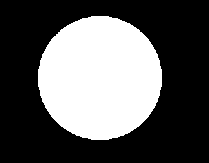
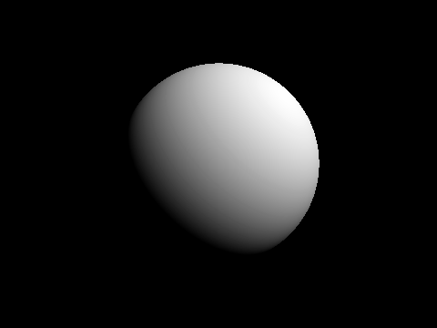
In this image, the sphere is at the position 0, 0, 50 with a radius of 15. The focal length is 350. This is pretty boring, so we can add diffuse lighting by instead setting the pixel’s color to the dot product of a light vector and the surface normal(we calculate that here). Here’s the new image with a light vector(unnormalized) of 1, 1, -1:
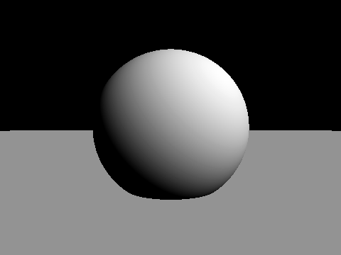
Next we can add a plane for one of the later articles, shadows:
Useful primitives
derpygamer2142, 26243AJ
A primitive is a basic function(in this case that returns distance) that can be used to construct more complex functions. You can find a full list of the functions that are being adapted at https://iquilezles.org/articles/distfunctions/
The arguments of this function are the point to find the distance to, the sphere’s position, and the sphere’s radius.
define Sphere sdf to point (x) (y) (z) sphere pos (sx) (sy) (sz) radius (radius)
    set [Sphere SDF return dist v] to (([sqrt v] of (((((sx) - (x)) * ((sx) - (x))) + (((sy) - (y)) * ((sy) - (y)))) + (((sz) - (z)) * ((sz) - (z))))) - (radius))
Advanced SDFs/SDEs
jfs22
Starting with a simple primitive, SDFs can be modified to create complex and organic shapes. I like to split these techniques into two categories, domain warping, and sdf warping
Domain warping
Domain warping takes in the ray position, and moves this position before calculating distance, effectively warping the domain, and the objects. The following transformations use this.
Stretching
Simple stretching along a coordinate axis can be done with a division. Stretching the Y axis by 2 times would be written as Ray Y/2, so in a function with an input of Ray Y, it would instead by Ray Y/2. This technique applies to all axes.
Shearing

Domain repetition
Isolating repetition
Noise
Sdf warping
These types of transformations modify the sdf, instead of the domain. By adding or subtracting to the sdf, geometry grows or shrinks, allowing the following transformations.
Displacement
Smoothing
Examples
Raymarched Normals
jfs22, 26243AJ
Raymarched Normals can be approximated with multiple SDF samples, or in specific scenarios, can be skipped by using the directional derivative method.
Solving the normal
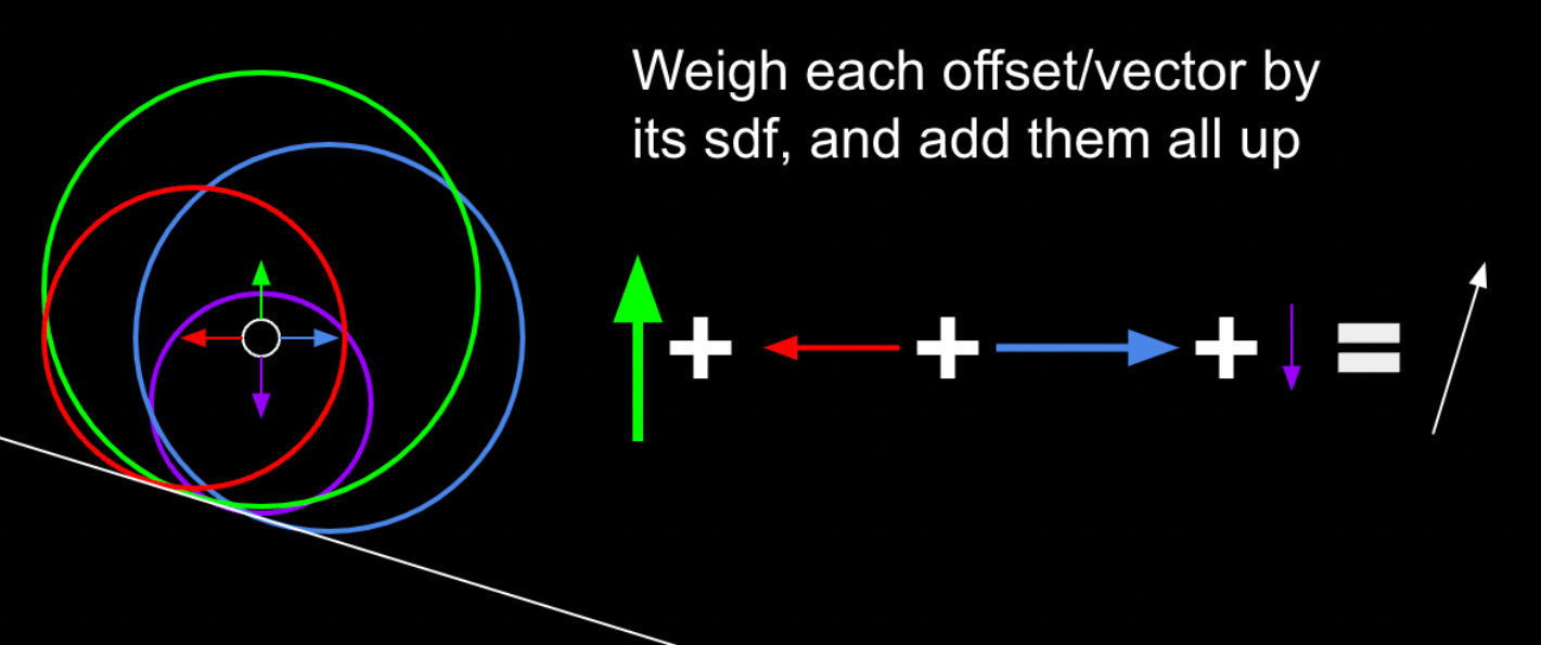
In raymarching, normals can be computed by sampling SDF values around a point. To see how this works, let’s first define a normal. Yes, normals are the direction of a surface, but what does this mean in terms of the SDF? We can see that moving the ray in the direction of the normal would increase the SDF by the greatest amount. Taking this logic, we can sample multiple points around the actual intersection point and see how the SDF changes, then create a vector which maximizes the SDF. In this diagram, you can see how samples pointing towards and away from the surface add to those components of the vector, and samples moving along the surface add less. By adding these up, you get an approximation of the normal.
In 3d, you can sample 6 points, one on each axis. This works, but is not optimal. Instead of sampling each axis, we can instead approach this problem by constructing a set of vectors where only one surface would be able to satisfy the sampled sdfs, which turns out to be 4 vectors in the shape of a tetrahedron. The code follows;
define get normal at point (x) (y) (z)
    Scene SDF ((x) + (0.001)) ((y) - (0.001)) ((z) - (0.001)) :: custom
    set [normal x v] to (SDF)
    set [normal y v] to (() - (SDF))
    set [normal z v] to (() - (SDF))
    Scene SDF ((x) - (0.001)) ((y) - (0.001)) ((z) + (0.001)) :: custom
    change [normal x v] by (() - (SDF))
    change [normal y v] by (() - (SDF))
    change [normal z v] by (SDF)
    Scene SDF ((x) - (0.001)) ((y) + (0.001)) ((z) - (0.001)) :: custom
    change [normal x v] by (() - (SDF))
    change [normal y v] by (SDF)
    change [normal z v] by (() - (SDF))
    Scene SDF ((x) + (0.001)) ((y) + (0.001)) ((z) + (0.001)) :: custom
    change [normal x v] by (SDF)
    change [normal y v] by (SDF)
    change [normal z v] by (SDF)
    normalize (normal x) (normal y) (normal z) :: custom
Advanced shadows
jfs22, derpygamer2142
Although not cheap, simple shadows can be done just by shooting a ray from the surface of an object towards any light. This checks for any obstructions between the light, allowing simple, hard shadows. If the point at the surface of the object is obscured, it is dark. If it isn’t, it’s bright. In code, it is a simple if statement checking if the ray has hit.
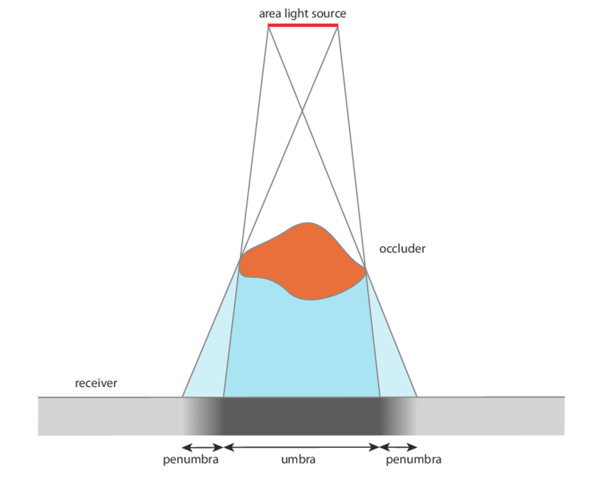
In reality, however, there is no particular line separating shadows, but instead a smooth transition between light and shadow. This gradient is called the penumbra, where not all of a light is illuminating an object. Although it’s impossible to calculate the penumbra in one ray, it can be approximated practically for free by storing the minimum of a simple division and multiplication. For each step of the shadow ray, (SDF/Distance of the ray)*Sharpness constant is compared to the current minimum, and set if it is smaller. This works since near misses slowly transition from the SDF factor and the distance causes further points to fade out more, like in real life. In code, this is run every step of the ray, inside the “for loop” shown earlier;
if <(((Sharpness) * (SDE)) / (Ray Length)) < (Shadow)> then
    set [Shadow v] to (((Sharpness) * (SDE)) / (Ray Length))
end
Once again, multiplying this lighting value by the color leaves a result similar to this:
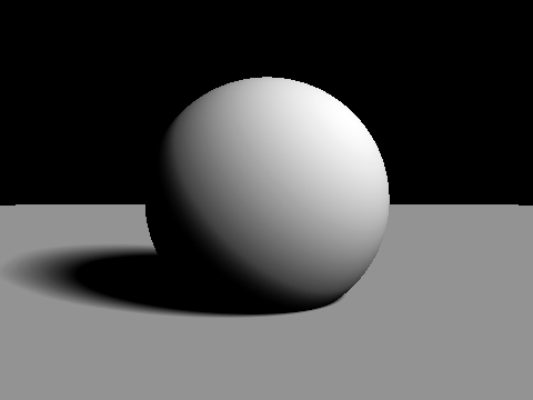
Ambient occlusion
jfs22
Ambient occlusion is one of many techniques used to replicate path traced graphics. This simulates ambient light being occluded by surrounding elements, often seen in corners. Taking advantage of our distance estimates, we can sample points at varying distances in the normal direction, and compare the distance estimates.
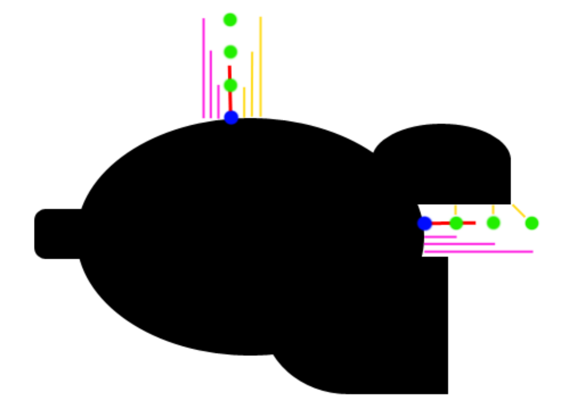
You can see how this works on the diagram on the right, where the yellow lines represent the distance estimates, and the pink lines represent the distance from the original point. In a perfectly flat section, the yellow distance is equal to the pink distance, but on occluded corners, you can see that the yellow distance is significantly less. We can model this by subtracting yellow from pink for each sample, adding them up, and multiplying by a value controlling the strength of the effect. You may notice however, that your ambient occlusion seems to be reversed. This is fixed simply by subtracting from one resulting in this:

Like above, k represents the strength of the ambient occlusion, while j represents how many samples you take. There is one last change to make, however. Using this model, far away samples contribute equally to the ambient value, which can leave unnatural results. You can optionally have further points contribute exponentially less to fix this, multiplying samples by smaller and smaller amounts as follows:

Path-tracing
badatcode123,bambozzle
Path-tracing, a subset of raytracing, is a way to make highly realistic images. Path-tracing emulates how rays of light behave in the real world, to give more realistic results than other rendering techniques at the cost of performance.
In the real world, rays of light are emitted from light sources, and bounce around the world until they hit your eyes. As the light ray bounces off objects, some of the frequencies of light in it get absorbed, tinting the light. However, in path-tracing, the rays are shot from the camera and bounce around the scene until it hits a light source (or some maximum bounce limit is reached, for performance reasons). This is because simulating rays from the light is wasteful, as most of these rays will not end up at the camera, and so will not affect the final image, but when the rays are shot from the camera, all rays are relevant to the final image. This is still accurate as light behaves the same whether it is moving forwards or backwards in time1.
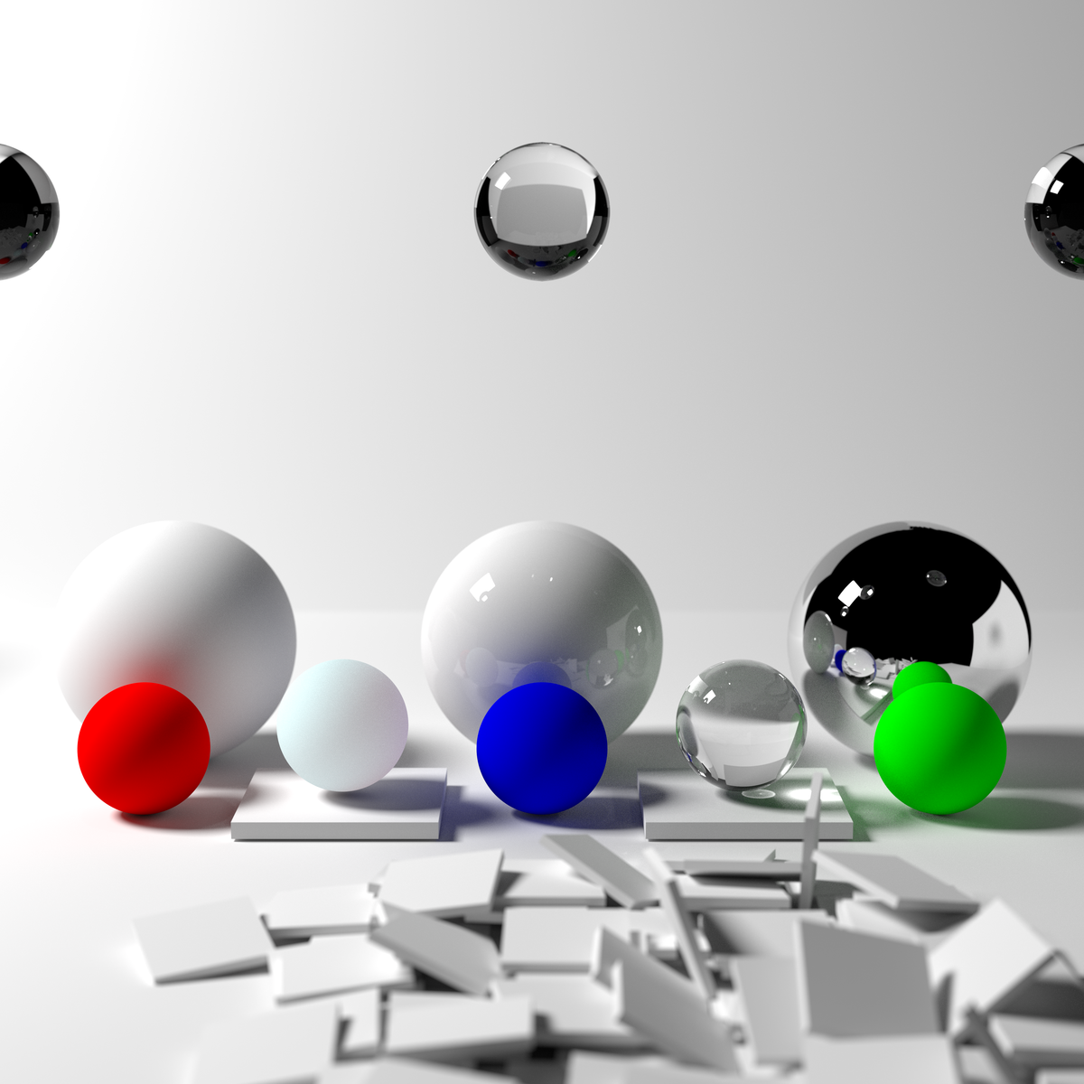
But before implementing pathtracing, let’s look at the rendering equation.
The rendering equation
The rendering equation is the equation all pathtracers try to approximate/solve. And it looks like this:
While this might look scary, it is actually incredibly simple. The equation pretty much tells us how much light a point on some object receives, it does this by shooting an infinite amount of rays in a hemisphere around the point, this is what the integral symbol and dwo represent, so we can ignore those. The following equation, then, gives how much light comes from some specific direction (radiance).
Now, we can look at the individual functions inside the rendering equation. Li represents the raw amount of light coming from some direction wo at point x (this function itself calls the rendering equation), the BRDF represents the percent of light that
For each object we need to know its color, emissive color (the color of the light it emits, set to 0 if it’s a light source) and whether or not it is a light source, alongside other properties related to its shape. We also need to know its surface normal so that we can shoot the ray from the intersection position correctly.
Now to implement pathtracing, we first need to get the surface normal. The surface normal of an object can be outputted by the intersection function itself. Then we need an emissive color for the lights. We need 6 new variables, named ray throughput r,g,b and ray emissive r,g,b. The ray emissive variables will be the final color of the pixels, while the ray throughput variables will be to store the colors of the objects the ray has encountered so far (for indirect illumination). So, for each object, define its emissive color, and make 6 new variables to store these properties (including the surface normal). Now, after each intersection we do this
- Change the ray emissive color by throughput*object emissive color
- Set the throughput to throughput*object color
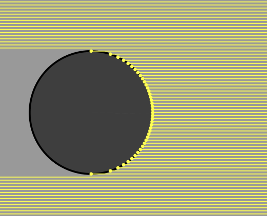
Make sure to set all the color channels in the throughput to 1 and the emissive’s to 0 before shooting the ray from the camera. We should also add a is light? boolean to the intersections to determine when objects are light sources and we can stop tracing the ray. We should also multiply the throughput by the dot product between the outgoing direction and the normal vector (see the math section), this is because light is more spread out at steep angles so there is less light hitting a particular point overall, this effect can be shown with the below image, we do the dot product with the outgoing direction rather than the incoming direction because we are doing the light calculations in reverse.
Here’s the code for the normal of a sphere and how to use it.
set [normal x v] to (((nx) + ((t) * (ray dir x))) / (rad::custom))
set [normal y v] to (((ny) + ((t) * (ray dir y))) / (rad::custom))
set [normal z v] to (((nz) + ((t) * (ray dir z))) / (rad::custom))
check if intersecting (t) object color (r::custom) (g::custom) (b::custom) object emissive color (er::custom) (eg::custom) (eb::custom) surface normal (normal x) (normal y) (normal z) light? <is light?::custom> :: custom
define check if intersecting (t) object color (r) (g) (b) object emissive color (er) (eg) (eb) surface normal (nx) (ny) (nz) light? <is light?>
    if <<(t) > (0)> and <(t) < (ray t)>> then
        set [ray t v] to (t)
        set [object color R v] to (r)
        set [object color G v] to (g)
        set [object color B v] to (b)
        set [object emissive r v] to (er)
        set [object emissive g v] to (eg)
        set [object emissive b v] to (eb)
        set [object normal x v] to (nx)
        set [object normal y v] to (ny)
        set [object normal z v] to (nz)
        set [is light v] to <is light?>
    end
With the surface normal we can make a simple diffuse sphere. Diffuse means that the outgoing ray direction is completely random, so we need to be able to generate a random unit vector, then check that this random vector is in the correct orientation (facing the same side as the normal), to do this, take the dot product between the normal and the random vector, if it is less than 0, we invert the random vector. We can then set it as the ray direction. We then shoot the ray again, but from the intersection point and the new ray direction. Make sure to move the ray to the intersection point before generating the new outgoing direction.
set [ray origin x v] to ((ray origin x) + ((ray t) * (ray dir x)))
set [ray origin y v] to ((ray origin y) + ((ray t) * (ray dir y)))
set [ray origin z v] to ((ray origin z) + ((ray t) * (ray dir z)))
define random on sphere
    set [t1 v] to (pick random (0.0) to (360.0))
    set [y v] to (pick random (-1.0) to (1.0))
    set [t2 v] to ([sqrt v] of ((1) - ((y) * (y))))
    set [x v] to ((t2) * ([cos v] of (t1)))
    set [z v] to ((t2) * ([sin v] of (t1)))
From SpinningCube
Now we can make a loop that represents the ray bounces, how many times it repeats is the amount of bounces around the scene the ray does. Defining a scene custom block can make it easier to edit and make the scene.
The ray bounces loop then looks like this:
repeat (5)
    set [ray t v] to (1000)
    scene :: custom
    if <not <(ray t) = (1000)>> then
        change [ray emissive r v] by ((throughput r) * (object emissive r))
        change [ray emissive g v] by ((throughput g) * (object emissive g))
        change [ray emissive b v] by ((throughput b) * (object emissive b))
        set [throughput r v] to ((throughput r) * (object color r))
        set [throughput g v] to ((throughput g) * (object color g))
        set [throughput b v] to ((throughput b) * (object color b))
        if <(is light) = [true]> then
            stop [this script v]
        end
        generate new outgoing direction :: custom
        set [dot v] to ((((ray dir x) * (object normal x)) + ((ray dir y) * (object normal y))) + ((ray dir z) * (object normal z)))
        set [throughput r v] to ((throughput r) * (dot))
        set [throughput g v] to ((throughput g) * (dot))
        set [throughput b v] to ((throughput b) * (dot))
    else
        stop [this script v]
    end
end
Now when rendering, it should look like this

However, this image is very noisy. This is because we are only sending one ray per pixel (1 sample), when we really should be trying to send as many as possible. There are 2 ways to do more samples, store the render in a buffer and keep rendering the scene and averaging the colors in the buffer and the colors in the render, or do all the samples at once using a repeat block, adding up the colors of the different samples and dividing by the amount of samples we took. We will be doing the second method since it is easier.
define get pixel color (x) (y)
    repeat (samples)
        set [ray origin x v] to (0)
        set [ray origin y v] to (0)
        set [ray origin z v] to (0)
        set [length v] to ([sqrt v] of ((((x) * (x)) + ((y) * (y))) + ((focal length) * (focal length))))
        set [ray dir x v] to ((x) / (length))
        set [ray dir y v] to ((y) / (length))
        set [ray dir z v] to ((focal length) / (length))
        shoot ray :: custom
        change [avg r v] by (ray emissive r)
        change [avg g v] by (ray emissive g)
        change [avg b v] by (ray emissive b)
    end
    RGB to decimal ((avg r) / (samples)) ((avg g) / (samples)) ((avg b) / (samples)) :: custom
Now we can easily decrease the noisiness of the image by increasing the sample count, at the cost of speed. Here is the same scene from before but with 20 samples
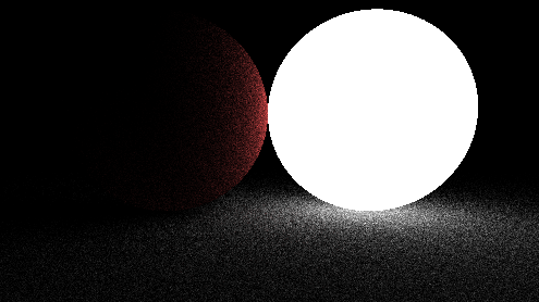
As you can see, the noise has decreased significantly and will decrease even more as the sample count is increased. But it takes quite a long time for the output to converge to an image that doesn’t have visible noise, to fix this we need to improve the way we are shooting out rays from the objects. In order to do this, we should first look at the rendering equation.
The rendering equation
The rendering equation is the equation all pathtracers try to approximate. And it looks like this:

While this might look intimidating, it is actually surprisingly easy. The integral with the Ω symbol is telling us to integrate over a hemisphere of all possible outgoing ray directions, so we can ignore the integral symbol and the dωo. Now let’s define the variables, the x variable represents a position in space, ωo represents the outgoing direction of a ray while ωi represents the incoming direction. The Li() function tells you the amount of light from x in some direction ωo, this function itself uses the rendering integral, which is why the rendering equation is recursive. The BRDF() stands for bidirectional reflectance distribution function, it essentially tells you the amount of rays going out in some direction based on the incoming direction. Here is a representation of the lambertian/diffuse BRDF
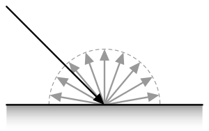
It is just a hemisphere because every direction has an equal chance to be picked. This is the specular BRDF
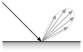
As you can see, it more light reflects specularly
The BRDF of diffuse materials is simply albedo/π, albedo means the amount of light reflected off of a surface. An albedo of 1 means the surface reflects all light that hits it and an albedo of 0.5 means the surface will absorb half the light and reflect the other half. Since we are always reflecting the light, we should be diving the throughput by π, but since we aren’t, we are implicitly saying that the albedo is π, which is wrong because no surface should reflect more light than the light it hits, to correct for this we must divide the throughput by π. The final term, (ωo*n) is just the dot product between the outgoing ray direction and the surface normal, and we are already multiplying the throughput by this.
Obviously, we cannot sample every direction in a hemisphere since there is an infinite amount of directions to sample, so to solve the rendering equation, a technique called Monte Carlo integration is used. A Monte Carlo algorithm samples a function at random values and averages these samples to approximate the true answer to an integral. Some integrals (such as the rendering equation) require many samples to converge, but given enough samples a Monte Carlo algorithm ALWAYS converges. However, there are ways to help the algorithm converge faster, one such method is called importance sampling.
Importance sampling
Importance sampling is a method that samples the most important part of an integrand and downsamples (makes it contribute less by multiplying the output by a small number) the samples to correct for the bias. For example take the function below
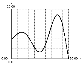
To importance sample this, we would sample more around the peaks and sample less around the valleys. There are many different areas we could importance sample in a pathtracer, however we will be looking at the easiest one for now. The multiplication of the throughput by the dot product between the surface normal and the outgoing ray direction can be worrisome because if the outgoing direction is almost perpendicular to the normal, the throughput will be multiplied by a very small number and the work of the ray will be essentially wasted, meanwhile if the direction is very similar to the normal the throughput will be multiplied by a number close to 1, if we could find a way to sample directions closer to the normal more often and perpendicular to it less often, we wouldn’t waste as much rays. This actually ends up being very simple to do, after generating a random direction, simply add the surface normal to it and then normalize the vector, now we can then remove dot product multiplication. However, this would actually double the brightness of all objects, thus we need to divide the throughput by 2, you could also just divide by tau instead of having to divide by pi then divide by 2.
After implementing this, our pathtracer immediately sees a jump in quality
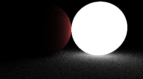
(same scene and sample count as before, but with a brighter light source)
We aren’t downsampling by much more because it turns out that biasing the outgoing direction this way almost perfectly cancels out the dot product. We won’t be providing a formal proof here, but you can find some online.
Known as the Helmholtz Reciprocity Principle
Sprite-Based Rendering
bigbrain123321
It is possible to use sprites to create 3D environments. When using Sprite 3D, objects will always appear to be pointing towards the camera regardless of camera orientation. For this reason the camera is often restrained from looking up or down. This method is simpler and faster than most other 3D techniques, as each object is treated as a point as opposed to a line or polygon. It is also possible to create a high level of textural detail with clever use of costumes. As such this method is widespread on Scratch.
Example of a sprite 3D engine
Overview
bigbrain123321
Sprite 3D engines work by storing the data of 3D points and by using the “stamp” tool found inside Scratch’s pen extension (at least for non-clone based engines but that’s for later). The 3D points are then transformed and projected and then corresponding sprites are stamped at the projected points. There are two ways to do sprite 3D: with clones or lists and stamping. Both methods have their own advantages and disadvantages. For example, clones allow for sprites to be a clear resolution while stamping slightly reduces a sprite’s resolution. However clone engines also tend to perform worse than stamp engines and have a max limit of 300 objects in vanilla Scratch (due to the 300 clones limit). It is important to note that Turbowarp (a Scratch mod that makes projects run faster) allows you to pass the 300 clones limit as well as the 200,000 list length limit. Typically it is best to use a stamp based engine but this chapter will go over how both methods work.
Stamp Based Engine
bigbrain123321
To create a stamp based engine all the object data needs to be stored in lists. This data includes the object’s position, its costume (sprite that will be stamped for it), and its size. Additional data can be assigned to an object such as ghost effect, brightness, etc. To do this the X coordinates can be stored in one list, the Y coordinates can be stored in another list, and the same goes for the Z coordinates, object costumes, etc.
Here is some example code demonstrating how you could go about creating and storing this object data:
define OBJECTS | add 2.5D sprite | x: (x) y: (y) z: (z) costume: (costume) size: (size) ghost effect: (ghost)
    add (x) to [OBJ: x v]
    add (y) to [OBJ: y v]
    add (z) to [OBJ: z v]
    add (costume) to [OBJ: costume v]
    add (size) to [OBJ: size v]
    add (ghost) to [OBJ: ghost effect v]
It is important to remember to delete all the data stored in these lists when the project is first run before you add new objects.
delete all of [OBJ: x v]
delete all of [OBJ: y v]
delete all of [OBJ: z v]
delete all of [OBJ: costume v]
delete all of [OBJ: size v]
delete all of [OBJ: ghost effect v]
Once we’ve gotten object creation done, we can now start talking about rendering these objects. First the 3D points that each object belongs to must be transformed around the camera using a rotation matrix. The transformed points will be stored in other lists (transformed x, transformed y, transformed z). Then the transformed points need to be projected into 2D coordinates that can be displayed on the screen. The projected points will also be stored in other lists (projected x and projected y). The contents of the transformed points lists and projected points lists need to be deleted every frame before transformations are applied.
Here is some example code:
delete all of [RENDER: tx v]
delete all of [RENDER: ty v]
delete all of [RENDER: tz v]
delete all of [RENDER: px v]
delete all of [RENDER: py v]
set [RENDER: index v] to (1)
repeat (length of [OBJ: x v])
    set [RENDER: temp 1 v] to ((item (RENDER: indx) of [OBJ: x v]) - (CAMERA: X))
    set [RENDER: temp 2 v] to ((item (RENDER: indx) of [OBJ: y v]) - (CAMERA: Y))
    set [RENDER: temp 3 v] to ((item (RENDER: indx) of [OBJ: z v]) - (CAMERA: Z))
    set [RENDER: x v] to ((((RENDER: temp 1) * (item (1) of [matrix v])) + ((RENDER: temp 2) * (item (2) of [matrix v]))) + ((RENDER: temp 3) * (item (3) of [matrix v])))
    set [RENDER: y v] to ((((RENDER: temp 1) * (item (4) of [matrix v])) + ((RENDER: temp 2) * (item (5) of [matrix v]))) + ((RENDER: temp 3) * (item (6) of [matrix v])))
    set [RENDER: z v] to ((((RENDER: temp 1) * (item (7) of [matrix v])) + ((RENDER: temp 2) * (item (8) of [matrix v]))) + ((RENDER: temp 3) * (item (9) of [matrix v])))
    add (RENDER: x) to [RENDER: tx v]
    add (RENDER: y) to [RENDER: ty v]
    add (RENDER: z) to [RENDER: tz v]
    add ((CAMERA: FOV) * ((RENDER: x) / (RENDER: z))) to [RENDER: px v]
    add ((CAMERA: FOV) * ((RENDER: y) / (RENDER: z))) to [RENDER: py v]
    change [RENDER: index v] by (1)
end
Once the points have been transformed, we need to sort the objects based on distance from the camera. This is to prevent objects that are farther away than being drawn over objects that are closer to the camera. To do this we can cycle through all the transformed point data and add the index of each point to a list (we can call this “sort ID” ) and the transformed z value to another list (this can be called “sort distances”). We use the transformed z value because it also represents the distance from the camera and it is faster to do this than using the distance formula. It is important that we only add this data to the sort ID and sort distances lists if and only if the point has a transformed z value that is greater than 0. This is so objects behind the camera don’t get drawn and produce weird artifacts. It is important to remember to delete the contents of the sort ID and sort distances lists before looping through the points to add them to these lists.
Here is some example code for what was just discussed:
delete all of [SORT: ID v]
delete all of [SORT: distance v]
set [RENDER: index v] to (1)
repeat (length of [RENDER: tx v])
    set [RENDER: z v] to (item (RENDER: index) of [RENDER: tz v])
    if <(RENDER: z) > (0)> then
        add (RENDER: index) to [SORT: ID v]
        add (RENDER: z) to [SORT: distance v]
    end
    change [RENDER: index v] by (1)
end
Once the objects have been prepared to be sorted, we can now sort the lists based on the objects’ transformed z values (distance from camera). Insertion sort or quicksort are fast sorting algorithms that we can use to sort the objects. It is important to note that when an item switches its index ( or place) in the sort distances list, the corresponding item in the sort ID list also needs to be moved to that same index in the sort ID list. This ensures that each object’s index in the sort ID list matches with its original transformed z value in the sort distances list.
Now we can get to rendering. Since the list with the objects’ distances are sorted from closest to furthest (closest objects are at the start of the list, farther objects are towards the end of the list) we can loop through that list starting from the last item all the way to the first item.
Here is some example code for a rendering script:
set [RENDER: temp 1 v] to (length of [SORT: ID v])
repeat (length of [SORT: ID v])
    set [RENDER: temp 2 v] to (item (RENDER: temp 1) of [SORT: ID v])
    set [RENDER: z v] to (item (RENDER: temp 2) of [RENDER: tz v])
    set [RENDER: temp 3 v] to (((1) / ((RENDER: z) / (CAMERA: FOV))) * (item (RENDER: temp 2) of [OBJ: size v]))
    switch costume to (BLANK v)
    set size to ((1) / (0)) %
    go to x: (item (RENDER: temp 2) of [RENDER: px v]) y: (item (RENDER: temp 2) of [RENDER: py v])
    if <(RENDER: temp 3) < (100)> then
        switch costume to (item (RENDER: temp 2) of [OBJ: costume v])
        set size to (RENDER: temp 3) %
    else
        set size to (RENDER: temp 3) %
        switch costume to (item (RENDER: temp 2) of [OBJ: costume v])
    end
    set [ghost v] effect to (item (RENDER: temp 2) of [OBJ: ghost effect v])
    point in direction (90)
    stamp
    change [RENDER: temp 1 v] by (-1)
end
In the code before going to the projected point that the object belongs to, the costume is switched to a “blank” costume (0 by 0 pixels) and the size is set to 1/0 (or “Infinity”). This is to allow stuff to go offscreen and that is important. The variable “RENDER: temp 3” is used to set the size of the object based off of the distance from the camera. Objects that are further away will be smaller than those closer to the camera (perspective).
Grids
Most 3D Engines are used to render arbitrary scenes - scenes where any 2 objects, polygons, points etc. have no defined relationship to each other. This gives greater flexibility, however there are some cases where greater performance can be gained by allowing certain assumptions. By far the most common is the rectilinear grid - grids constructed from squares (or voxels in the 3-dimensional case). The properties of grids allow major optimisations to be made in both projection- and ray-based engines.
Projection
26243AJ
Directly rendering a voxel world with projected voxels is a powerful technique that allows for realtime* minecraft-like games. By constricting the world to a grid, we can take advantage of many properties of ordered voxels in order to create exceedingly fast rendering engines, vastly surpassing the maximum triangle count for many other polygon-based 3d engines.
Using rotation matrices to optimize projection
The rotation matrix is the cornerstone of projection-based 3d engines. However, polygon-based 3d engines are only able to make use of some of the potential of this matrix.
Although it is natural to think about a rotation matrix as one whole operation which converts worldspace coordinates to cameraspace, when applying the matrix to a grid, it is easier to treat said matrix as a set of individual vectors.
What is a coordinate?
In an unrotated 2 dimensional space, coordinates represent a scale factor applied to 2 vectors. The x coordinate would represent the scale factor of the vector (1, 0), the y coordinate would similarly represent the scale factor of the vector (0, 1), and combining these scaled vectors would result in the final point in space. For simplicity, these vectors will be represented as V.x and V.y respectively. Thus, a coordinate value of (x, y) would be converted into a position in space, represented by P, through the equation P = x*V.x + y*V.y.
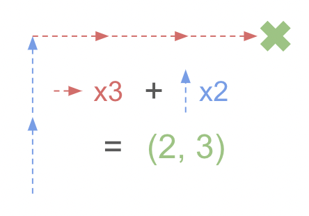
The rotation matrix modifies these initial vectors, replacing them with their rotated counterparts. This, in turn, rotates the point.
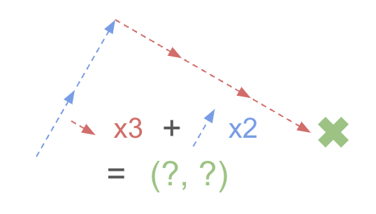
Things become interesting when we move the original point across the two axes, creating a grid.
For example, let’s rotate a line parallel to the x axis formed by a list of coordinates (x, y), (x + 1, y), (x + 2, y), and so on. Applying the operation from above, this would result in a set of points (x*V.x + y*V.y), ([x+1]*V.x + y*V.y), ([x+2]*V.x + y*V.y), and so on. Interestingly, once the initial point has been calculated, the rest of the points can be calculated by simply adding a single vector. If we define our initial point as O = (x*V.x + y*V.y), the next point could be simplified down to O + V.x, and this can be repeated for the rest of the points. By doing so, we are able to reduce an entire matrix multiplication operation for each point down to just a few additions.
This can easily be applied to 3d grids by using a set of 3 3d vectors which represent each axis.
Calculating these vectors is also fairly trivial, as these can be directly obtained from the rotation matrix. By expanding out the matrix into an equation for each axis, we can determine that each column of the rotation matrix equates to the 3 3d vectors we mentioned before.
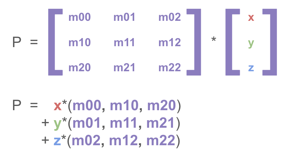
The code implementation of this is shown below, assuming that the rotation matrix has been constructed beforehand and is used like so:
(refer to Rotation Matrix for the construction of this matrix)
define rotate point (x) (y) (z)
    set [rotated x v] to ((((x) * (item (1) of [rotation matrix v])) + ((y) * (item (2) of [rotation matrix v]))) + ((z) * (item (3) of [rotation matrix v])))
    set [rotated y v] to ((((x) * (item (4) of [rotation matrix v])) + ((y) * (item (5) of [rotation matrix v]))) + ((z) * (item (6) of [rotation matrix v])))
    set [rotated z v] to ((((x) * (item (7) of [rotation matrix v])) + ((y) * (item (8) of [rotation matrix v]))) + ((z) * (item (9) of [rotation matrix v])))
Each axis is defined recursively, which simplifies the code
A projection onto the 2d screen is also required, which can be calculated by multiplying the rotated x and y coordinates by FOV/z.
Here is an example of how to render these points:
define render point (x) (y) (z)
    go to x: ((((x) * (FOV)) / (z))) y: ((((y) * (FOV)) / (z)))
    set pen size to (((0.1) * ((FOV) / (z))))
    pen down
    pen up
By combining this with some camera movement code, you will be able to explore a grid of points. You may also want to add z culling, as points behind the camera can appear massive and obstruct your view.
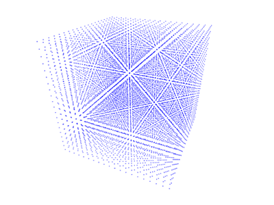
Octant Sorting
26243AJ
Although rendering the points is fairly simple, efficiently sorting them is another challenge.
It is possible to just input the points into a regular sorting algorithm, and then render them accordingly, however this scales very poorly with the number of points needed to sort for grids (the final render in the previous section contains 8,000 points, and it’s only a 20x20x20 grid).
Octant sorting and its variants overcome this scalability by simply traversing the grid in a certain order, so that all points are correctly sorted. This makes this sorting algorithm an O(n) algorithm, making scale significantly better than other sorting algorithms which commonly range from O(nlog(n)) to O(n^2).
How sorting is done
Similar to many other methods used for 3d graphics, things become simpler and much more manageable when converted to 2d.
By drawing out a heatmap for a 2d grid, we can formulate the order the cells would need to be drawn in order for there to be no sorting errors.
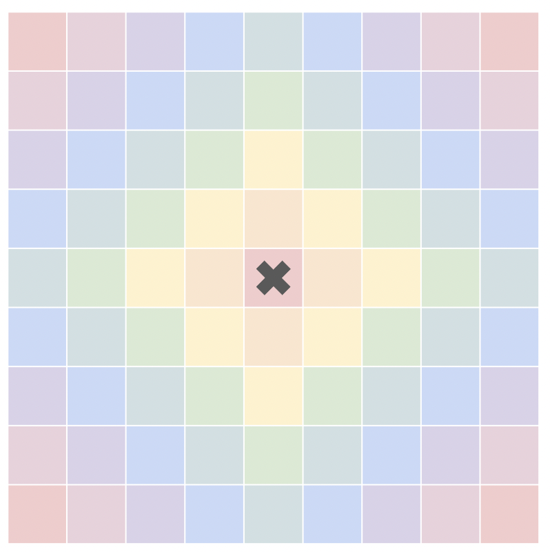
For there to be no sorting errors, the outermost red cells must be drawn first, and then the pink, purple, blue, and so on. This is possible, however there are much simpler options which result in almost identical results.
Instead of traversing the grid in a ring-like pattern, we can instead split the grid into 4 quadrants, and then traverse each of them from back to front. Doing so results in perfect sorting whilst still keeping the algorithm relatively simple.
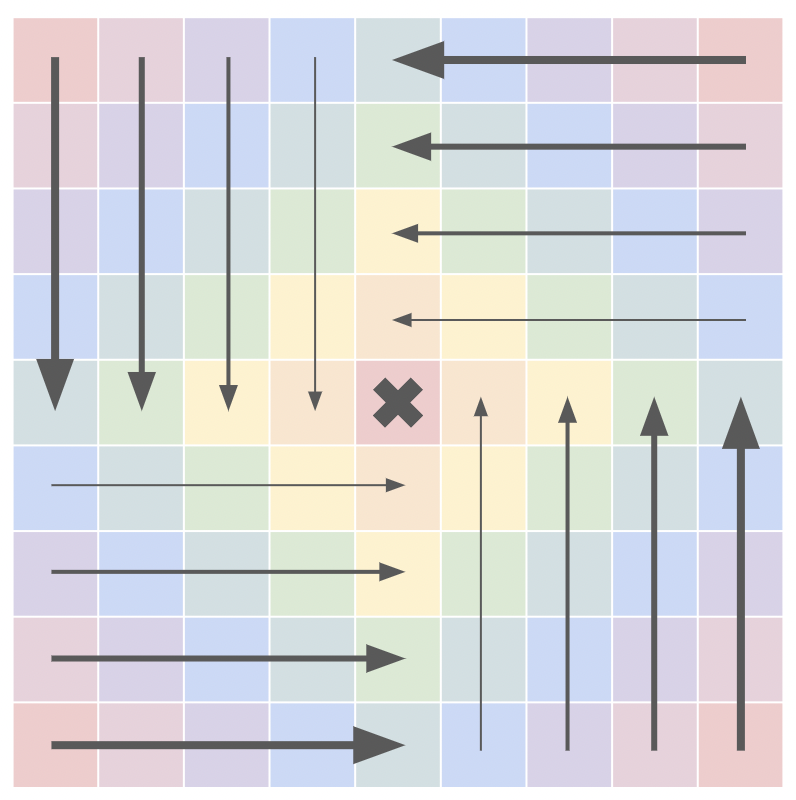
Shading
Badatcode123, SpinningCube, Robostew
Material
Diffuse objects are objects that reflect light completely randomly, meaning the outgoing and incoming directions have no relationship. This is often called lambertian reflectance.
Metals are objects that reflect light almost always in a specular way, meaning they often absorb transmissions.
Glasses usually refract light, but can also reflect light (more noticeable at steep angles, due to the fresnel effect).
Diffuse models
Many models, or BRDFs, exist for diffuse calculations, the most easiest and basic one is the lambertian diffuse model, it is defined simply as albedo/pi, with albedo being the reflectivity of the object. Other, more advanced models such as oren-nayar can represent diffuse objects more realistically at the cost of being more expensive to calculate and also needing many samples to converge because they use the microfact model.
Specular models
Diffuse models represent light that hits a surface and scatters in many directions due to small imperfections in the surface. It is common to include another type of lighting as well: specular lighting. This represents light that reflects as so:
The angle formed by the incoming ray and the surface is called the angle of incidence, and the angle formed by the reflected ray and the surface is the angle of reflection. These angles are the same for specular reflections.
If the reflected ray is pointing right at a light source1, then, by the Helmholtz Reciprocity Principle, much of the light from that light source would be reflected off the surface and back towards the incoming ray’s origin.
This should cause a very bright area on the surface. Indeed, you can observe this in real life (go outside, touch grass, etc.) by taking any shiny object and looking for the reflection of lights on the object. These bright areas are called specular reflections, and they can look very sharp or kind of blurry depending on how rough the object is.
I am using rays and the concept of reflected light here, but this effect can be achieved with typical rasterized renderers.
For a simple specular reflection:
- Find the incoming vector (the vector from the camera to the point you are shading).
- Reflect that vector across the surface normal.
- Normalize the reflection vector.
- Take the dot product of the reflection vector with the vector to a light source (normalized). Clamp this value to the range 0-1 to discard negative values.
- Raise this value to a power. Higher powers will result in sharper specular reflections.
- This value represents the intensity of the specular highlight cast by a light on a surface.
Many models for specular reflections exist. Real time graphics in scratch usually use a simple model like the Phong Reflection Model.
Or any other bright object or surface, although often only lights are considered
Combined
In graphics, it is common to combine both the specular and diffuse models, alongside the ambient value, for more realistic shading than just using one model, as seen below

By SpinningCube
Shadows
Ray-based
Hard shadows can be achieved by shooting rays directly at the light sources from an object’s surface. If the ray is blocked by some object before reaching the light source, that point on the surface is in shadow.
Raymarching can make an approximation of soft shadows, explained in the raymarching section.
Depth-buffer based
Another method of shadow casting is rendering the scene to a depth buffer from the light’s point of view. Then, when figuring out if a pixel is in shadow, we find where the pixel is in the depth buffer of each light, and if there’s a depth value smaller than the depth value of the current pixel, projected onto the depth buffer, then we can safely conclude that it’s in shadow. This method however, can be quite costly, because of the fact we need to render a depth buffer for each light source, plus to get a good shadow resolution, the resolution of each depth buffer has to be quite high. Keep in mind that for point lights, the fov of the theoretical camera on the light will be 360 degrees, which will add to the resolution of the depth buffer. Plus, rendering an image for each light is just not possible considering the limitations of scratch or turbowarp, unless the scene is very simple and there’s only a couple of lights.
Rasterizer
WIP => talk about how to do shadows with rasterizers.
Baked lighting
WIP => about baked lighting methods in Scratch (texture based like The Mast by awesome-llama, polygon-based like Sub 1k Block Challenge by littlebunny06)
Handling colors in Scratch
scratchtomv
In 3D computing, colors are often represented as a set of 3 values: Red, Green and Blue. There’s sometimes also a fourth one: Alpha (abbreviated as A), often used for transparency.
When rendering a 3D scene, these values can be easily modified to change the final color of the object. This is done through setting a Material color, Shading and Post-processing.
Color representation in Scratch
scratchtomv
Scratch supports the following color formats :
- Hexadecimal (ex: #FF2D55, 0xFF2D55)
- Decimal (ex: 16711680)
In scratch we’ll mainly use the decimal version as it’s faster to compute and takes fewer bytes in Scratch memory.
The pen color can be set with this block :
set pen color to (some color)
Or with the combination of these blocks (uses the HSVA model, and is slower) :
set pen (color v) to (50)
set pen (saturation v) to (50)
set pen (brightness v) to (50)
set pen (transparency v) to (50)
Color conversions
scratchtomv, jfs22, badatcode123, 26243AJ
RGB to decimal:
define RGB to Decimal (R) (G) (B)
    set pen color to ((round (B)) + ((256) * ((round (G)) + ((256) * (round (R))))))
RGBA to decimal:
define RGBA to Decimal (R) (G) (B) (A)
    set pen color to ((round (R)) + ((256) * ((round (G)) + ((256) * ((round (B)) + ((256) * (round (A))))))))
Hex to decimal: (Scratch/JS will automatically do the conversion)
define HEX to Decimal (HEX)
    set pen color to (join [0x] (HEX))
Post-processing
jfs22, badatcode123, 26243AJ
Post processing algorithms modify screen colors after all other effects, directly before rendering. These algorithms include tonemappers, gamma correction, color grading, and other color processing effects.
Tonemapping
Tonemappers can change the tone of the image, since it directly affects the colors. Tonemappers are also used to increase the white point/remove it all together (the white point is when a color that is too bright turns white because of clamping). A few popular tonemappers used in scratch can be found below.
https://www.desmos.com/calculator/fzixe9wazx
Gamma correction
Contrary to linear representations of colors, such as RGB, the human eye perceives brightness in a non-linear way. Our eyes are much more sensitive to changes in dark colors, and less sensitive to changes in bright colors. Thus, if we attempt to display a linear spectrum, to our eyes it will appear non-linear.

With a linear display and only 8 bits per color channel, banding artifacts in the dark images would be more noticeable—without enough dark shades to create a smooth transition, our eyes would pick up on the harsh edges. To combat this, most modern displays apply a gamma function to the input RGB colors to create a more balanced spectrum. This perceptual linearity reduces those color banding artifacts, affording greater color depth to dark parts of images. The specific function to use is defined in a color representation standard called sRGB, which is standard for nearly all imagery on the web (including all colors Scratch can output), and is widely adopted by consumer displays.

Although this is great news for our eyes, lighting calculations in 3D graphics must be done with linear RGB values to achieve physically accurate results. Thus, in order to produce accurate colors, when sampling an sRGB color/texture, we first need to convert it to linear RGB. This can be done by raising the color values to the power of 2.2. Likewise, when displaying linear RGB values, we need to convert them to sRGB by raising them to the power of 1/2.2. These calculations assume RGB values represented in 0 to 1 range.
Note that this is technically only an approximation* of the actual sRGB transfer function, the full conversion can be found below
https://www.desmos.com/calculator/5kppnk4gkx (by SpinningCube)
Using the exponent workaround, we can apply the x^(1/2.2) adjustment on Scratch:
define gamma correction (R) (G) (B)
    set [output R v] to ([e ^ v] of (([ln v] of (R)) / (2.2)))
    set [output G v] to ([e ^ v] of (([ln v] of (G)) / (2.2)))
    set [output B v] to ([e ^ v] of (([ln v] of (B)) / (2.2)))
If speed is a concern, sqrt(x) can be used instead of x^(1/2.2) for a rougher approximation.
*x^(1/2.2) is a very close approximation, quite common in game development, and even display manufacturers will often cheat by using x2.2 instead of the actual sRGB standard EOTF curve.
Color grading
Like other post processing effects, color grading changes the colors of an image, although it is usually done artistically, and for no physical reasons. One example of color grading is posterization or quantization, this stylization method lowers the range of colors that are displayed. This effect is sometimes used with dithering to trick your eyes into thinking there is more color ranges in the images (there is only pure black, or pure r,g or b in this picture).
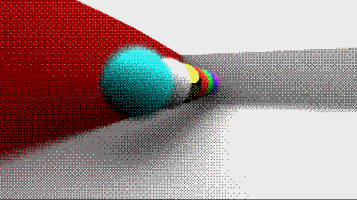
Binary Space Partitioning (BSP)
littlebunny06
littlebunny06’s Ramblings on BSP: The Undiscovered Country
Around the start of the COVID-19 pandemic, certain spheres of technical discussion materialized, and with this, technical developments. The Ray Madness studio appeared to curate raycasting projects. Many creators started creating. Around this time in 2020, a few brief and speculative mentions of this algorithm, BSP, appeared. I first saw mention of it from CubeyTheCube(Raihan142857). From there, I stumbled into Vadik1’s “perfect sorting” 3D engine. It had the ability to accurately sort intersections. It used BSP.
How Vadik1’s Algorithm Worked
Per every frame in the project, a custom block is called to operate on a list containing indices to each polygon in the scene. By selecting the first polygon on the list, it categorizes the other polygons into two groups: on the same side of the player(in front of the selected polygon), and on the opposite(behind).
These groups are formed within the original list(in-place), with same-side-to-camera polygons placed on one side of the selected polygon index in the list, and opposite polygons to the other. The start and end indices for these groups on the list are stored, and recursively passed into the custom block again, allowing the same process to occur on the sub-groups. This recursion terminates whenever a group has only one item left.
If you, the reader, have ever worked with comparison sorts, you may notice that this algorithm is some sort of partition-exchange sort(quicksort). It does indeed work quite like quicksort.
Here are the steps for an in-place quicksort algorithm:
- If the range has only one element left, stop the sub-routine(custom block)
- Otherwise, pick a value from within the range. This will be used as the pivot for the partitioning step.
- Partition by swapping the elements in a way so that all elements with values less than the pivot go before it, while elements with values bigger than the pivot come after it. Elements with values that are equal to the pivot can go either way. These swaps occur all-the-while keeping the pivot element’s position, which might move around during this step.
- Recurse the algorithm from the beginning of the sub-range up to the point before that of the division. Apply it to the sub-range after the point of division as well.
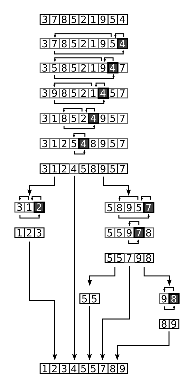
(From Wikipedia) Example of the Quicksort Algorithm on a random set of Numbers
So, Vadik1’s sorting algorithm works quite like a quicksort, only that instead of comparing values, the side which a polygon lands relative to a pivot polygon determines which group it falls into.
One thing which has been left out of this explanation, and that the reader may have noticed by now, is that some polygons are on both sides of a pivot. Vadik1’s algorithm deals with this by creating two new split versions of such polygons. These split versions are added to a separate, temporary list of polygons. This list is deleted upon each frame.
This algorithm produces a perfectly ordered list of polygons that can be rendered back-to-front in order to produce a perfectly sorted scene, even in the case of polygon intersection.
The code to this project, as well as Vadik1’s own description of how it works, can be found in this Scratch link: https://scratch.mit.edu/projects/277701036/
More Ramblings on BSP: The Traversal Into Rough Country
BSP Had Reached Its Limits
BSP was still an undiscovered country among the Scratch enthusiasts of 3D. As I dabbled into Vadik1’s code to produce my own 3D engine built on this concept, I had no idea what I was truly going to get myself into. Very soon, I entered a rabbit hole of graphics effects based on the idea first presented by Vadik1. I made the second iteration of Gamma Engine. It featured accurate polygon ordering with intersection support, and soon later, various graphics effects that relied on clipping volumes by using partitioning. By then, a couple more Scratchers were starting to pick up on the idea of BSP.
One of the big issues with this algorithm is that it’s slow. It's time-consuming to partition all the polygons and it stacks up as there are more numbers of them. Another issue is that, especially without any optimizing functions to help reduce split surfaces, certain scenes can cause a large buildup of split polygons after partitioning.
As I genuinely thought the limits of BSP had been reached, a Scratcher—Chrome_Cat—sought to solve these issues. After reading literature on the canonical implementation of BSP, he found his answer.
Then, There Were BSP Trees
A tree can be used to store the pivot polygons in each node. Upon each partitioning step, a new node is added to build this tree. The end result is a BSP tree, which can be traversed in linear time, in respect to the camera position, to access each node in correct render order. Chrome_Cat presented an algorithm that does such, and with the assertion that BSP trees could make the fastest 3D engine. It generated a tree in a compilation step, then traversed it on each frame during runtime. His 3D engine was indeed quite fast. It scaled up well. Within the generation function was a greedy pivot selection algorithm which looked through the range of polygons for one that would generate the least amount of splits. This allowed for massively reduced split counts on models.
Just as many of the fastest of all 3D engines of Scratch did not seem to have any significant room for optimization, this new idea was a breakthrough which, if not challenged the idea that 3D engines couldn’t be much faster technique-wise, brought new advances to a seemingly stagnating field. This however was the step into, what was at that point, the rough country of BSP as a technique.
I was also working on a 3D engine of my own alongside Chrome_Cat’s. This engine—the third iteration of Gamma Engine—also featured BSP trees. As I got further into the development of this Gamma Engine iteration, I would slowly find out that what I thought was all there was from the concept of BSP, was totally completely limited in actuality. But that will be a story for after we get a good idea of how a BSP tree is built and how it works on a conceptual level in Scratch.
Building A BSP Tree
Although the 3D implementations of BSP are 3D, of course, I will discuss 2D BSP trees for this explanation. This is because the principles of the 2D BSP tree which uses line segments extends to the 3D BSP tree which uses polygons.
The below figure shows a set of four segments that constitute the scene. We want to split the world into two, and each part into two, and so on, in such a way so that each segment resides in its own unique subspace. There are unlimited ways to do this so the question is: How would we want to do this?
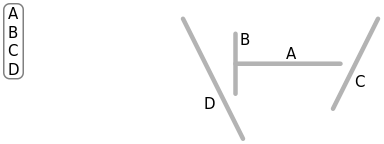
(From Wikipedia) A sample set of line segments in 2D space, and a list of the segments.
The simplest way is to simply split the world along the lines of the segments themselves. Each node would contain the wall that splits this scene. This is to be done recursively until a unique subspace boundary is created for each segment. This spatial organization provides an unambiguous visibility ordering explained earlier with Vadik1’s algorithm. This can be seen further as we get to the traversal step later.
The first step in this process takes the splitting line from segment A, and groups the world into two parts, walls that are in front, and walls that are behind, just like what was explained with Vadik1’s algorithm.
A node is created, and segment A is added to the node. The actual implementation details will be explained in the Scratch implementation section next.
An issue with choosing A as the splitting line is that there aren’t actually any segments which are wholly in front or wholly behind A. So as you might remember, the solution is to break B, C, and D into B1, B2, C1, C2, D1, and D2 along the splitting line.
The remaining segments are grouped into the list of segments in front of A(B2, C2, D2), and those behind (B1, C1, D1).
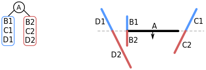
(From Wikipedia) The initial split along the line of segment A.
The algorithm is applied to the list of segments in front of A(B2, C2, D2). The front list is always processed first. Segment B2 is chosen and it is added to a new node. It splits D2 into both D2 and D3. Note that the new D2 is a split version of the old D2. D2 is added to the front list. C2 and D3 are added to the behind list.
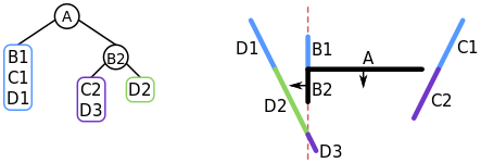
(From Wikipedia) The split on the list of segments in front of A. B2 is chosen in this step.
D2 is chosen and added to the node. Since it's the only one in its list, we stop there.

(From Wikipedia) D2 is chosen and added to a node in front of B2. It is the last item, so nothing further needs to be done.
As we are done with the lines in front of the node containing B2, we start looking at the list of segments behind it. C2 is chosen and added to a new node. The other segment, D3, is added to the list of lines in front of C2.
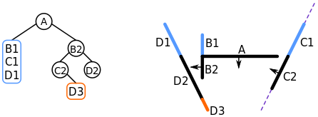
(From Wikipedia) C2 is chosen and added to a node behind B2.
D3 is added to a node. We stop here as it is the last segment in its list.
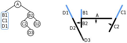
(From Wikipedia) D3 is chosen and added to a node in front of C2.
Since all of the segments in front of A have been added to their own respective nodes, we recurse on the list of segments behind A. We choose B1. It's added to a node and C1 is put into the behind list, D1 into the front list.

(From Wikipedia) B1 is added to a node, and C1 and D1 are grouped into their respective lists.
Finally, D1 is added to a node, then C1. The BSP tree is complete.


Now the BSP tree has been built, but it might not be immediately intuitive on how it helps with visibility ordering at all.
Movement
Rinostar
Basic Kinematics
First, it makes sense to know how objects move. Every physics object has a position and a rotation, obviously. Right now we’ll only look at position, because rotational kinematics is just a more complex version of regular kinematics. For every position, there’s also velocity, that describes how much an object moves. This is a vector quantity. Written in math terms, where p(t) is the final position at time t, and v(t) is velocity at time t, it would look like this:
p(t) = 0tv(t)dt .
Basically, this just says that the position changes based on velocity over time. Now, then there’s acceleration which describes how much the velocity changes. It’s also where the forces and different interactions get applied at. Same deal, a(t) is the acceleration function, it’s just:
v(t) = 0ta(t)dt .
Next up, force. Each object exerts some amount of force to other objects. The equation is simply F=ma. Force is also a vector. Since acceleration is a function, we make a = a(t), where t is the variable for time.
This code sample is just in 2d for simplicity purposes. In 3d, it’s the exact same, just with an added z component. The y on the acceleration is set to be -9.81, which exerts a constant force downwards, which you guessed it, is gravity.
Collision Detection Algorithms
There are multiple types of collision detection algorithms, which can be categorized into two types: broad phase, and narrow phase. For the most part, the algorithms you might hear the most are AABB, and SAT. AABB is a broad phase detection algorithm. SAT is the opposite; a narrow phase detection algorithm. Broad phase type algorithms are generally pretty simple and run pretty fast, but have low accuracy. Narrow phase type algorithms are, of course, the opposite. They generally are more advanced, being more accurate, but they’re a bit slower.
AABB Collision Detection Algorithm
AABB stands for Axis Aligned Bounding Box, which should give away some of how this thing works. All it does is to check if two axis aligned boxes are colliding, or inside of each other.
The disadvantage of this algorithm is that it can’t check any rotated boxes (non-axis aligned), so if you were to put a box collider on two objects, they can’t be rotated to the orientation of each object.
So with that out of the way, here’s how it works. If you squash two boxes onto a 1d line, like the x axis, they look like two lines, with a start and end point for each one. If we only think about this 1d line, we can see that if the two lines are intersecting, then the boxes are possibly intersecting.
(Illustrations done by Rinostar)
The equation for this is: Av1xBv2xAv2xBv1x . Now, for the y axis. To test if they’re intersecting or not, we need to also check for the y axis.
The equation for the y axis is this: Av1yBv4yAv4yBv1y. Similar to the x axis, but instead we will be using the fourth point for the y difference (height)1.
Putting all this together, it would look like this: (Av1xBv4xAv4xBv1x)(Av1yBv4yAv4yBv1y).
If your boxes had width and height, instead of points, it’s pretty easy to calculate the points.
For example, take this box, which has 4 points:
Let’s make v1 be the origin of the box. If we want to calculate v2 , the equation (w being width), would be: v1x+w, v1y. If we want to calculate v3 , (h benign height), it would look like v1x, v1y+h. For v4 it would be, v1x+w, v1y+h. Putting all this together in scratch as a custom block, it would look like this (v1 being the origin, v2 being (v1+w,h)):
For 3d, you’d use the z component, instead of the x or y, but it’s still the same check, with another if statement inside the two. So for any two bounding boxes, we’re now able to check if they’re colliding or not. But what about orientation, or other polygons, besides boxes?
SAT Collision Detection Algorithm
Here, we get to the good stuff: more precise and complex algorithms to tear your hair out trying to implement. Take two rotated boxes, just for simplicity. The summary of this algorithm is: if they’re not colliding, you can just draw a straight line through the two polygons, and none of the edges intersect. That’s why SAT is called “Separating Axis Theorem”.
So how do we find the separating axis? Well first, to actually implement this thing, we will have to check both polygons, switching which polygons are a and b in the second iteration. Inside that, we must check all the edges of polygon A, making a potential separating axis from each edge. How do we make a potential separating axis? Well, the separating axis can be calculated using just the normals of the current edge.
If v1is the start of the line, and v2 is the end of the line, This can be calculated like this: n=-(v2y-v1y), v2x-v1x .
As you can see, the normal is perpendicular to the current edge in the loop, which would be V1V2, or line AB. Next, we must project all the points of both polygons onto this line. If you don’t know already: it’s dot product time!
Taking the dot product of all the points, we must find the min and max points of both polygons to do a comparison similar to AABB on one axis. To do that, we must loop through all the points projected to the line and check if that point is less than the min point value, or greater than the max point value. In this example, Av1 = Amin, Av3=Amax, Bv4= Bmin, and Bv2=Bmax 2. Now, we can check if both polygons could be intersecting, using a bool equation: Amin Bmax Amax Bmin. If it returns false, then we stop the loops and conclude that they aren’t intersecting. If it returns true, we will continue iterating through the loops, and if we reach the edge and the bool equation still returns true, then we can conclude that the shapes are overlapping. You may ask, “Could we possibly get collision data, such as the normal, or min depth of collision from this?” The answer is yes! It is easier in SAT than AABB, as most of the variables needed for this are already here. For the normal, you just have to normalize the axis of projection. Then, for the depth of the penetration, just get the difference between the min of the projected polygon A point, and max of polygon B’s projected point. Now, it’s time for the more fun stuff: solving these collision cases.
You can use the third point for just the y, too.
If going down and right makes the dot products larger. It would be the opposite in min and max if it was the other way around, but it doesn’t really matter, it’ll still check fine.
BVH
BVH, or bounding volume hierarchy, is an acceleration structure that can speed up many algorithms such as collisions, raytracing, BSP tree construction etc. It uses a bounding volume, such as an AABB or a sphere, to contain objects, and then contains the volumes containing objects, hence the hierarchy. The leaf nodes represent the meshes, but can contain more than one object, this is done because usually it isn’t fastest to go that deep into the tree.
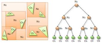
A BVH tree can be any type of tree, but we will be implementing a binary tree here. There are 2 ways to construct a BVH tree, bottom-up and top-down. Bottom-up method makes an AABB around every object in the scene, then connects 2 boxes that are close together, and makes boxes around that, this is repeatedly done until there is only one AABB left which covers the whole scene. Top-down makes an AABB around the entire scene, then chooses a splitting plane to split the scene into 2 regions, it then takes the maximum bounding box in those 2 regions, and repeats the process until every object has its own bounding box.
Construction
For bottom-up, we need to first make a “constructor” list that will be used to construct the tree, for this we need to loop over every object in the scene and find its minimum bounding box, we will be defining AABBs using their minimum and maximum vertex. The minimum bounding box of a sphere can be defined by adding the radius to each component of its position vector for the maximum vertex and subtracting the radius for the minimum vertex and then adding these AABBs to the constructor list, also adding it to a list representing the tree . We then combine the closest boxes together and add those to a different list.
Traversal
Traversal is the same in both methods, make a traversal custom block that has an input for the current node index, when starting traversal just set the index to the index of the root node, then test if the ray intersects with the root node, if it does, recurse down the left and right child nodes by calling the function again, but setting the node index to the index of the left/right child. You can make this faster by prioritizing the closer node first, this is because if the closer AABB happens to be hit, then you won’t have to traverse down the other AABB node, which can save a lot of time. Once the leaf node has been reached, do the intersection tests and simply don’t call the traversal function.
Math functions
Porting most of the functions from
https://www.khronos.org/opengles/sdk/docs/manglsl/docbook4/
Scratch doesn’t include a lot of useful mathematical or vector manipulation functions like in other programming languages. Here is a useful list of common math functions written in Scratch code :
Dot product: tells how alike 2 vectors are, if they are the same length. 1 means they are the same vector and -1 means they are the exact opposites, and 0 means they are perpendicular to each other.

Exponents: repeatedly multiplies x by itself y times.

Cross product: gives a vector perpendicular to the 2 vectors inputted.
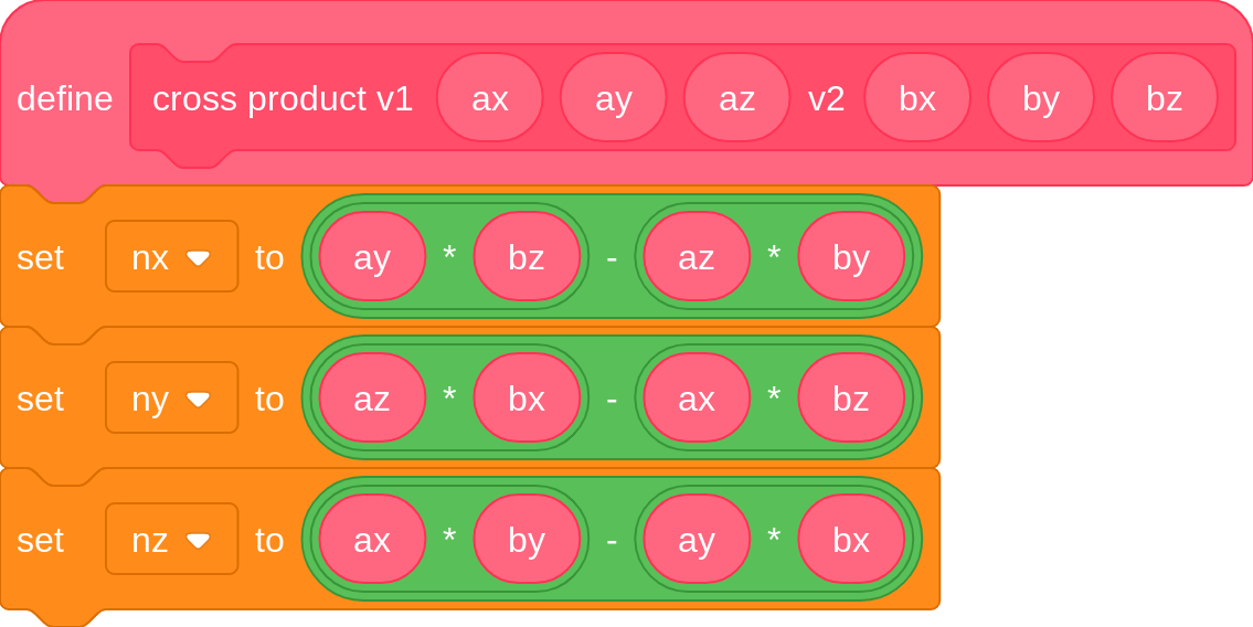
Test if triangle is ordered clockwise : (useful for backface culling)
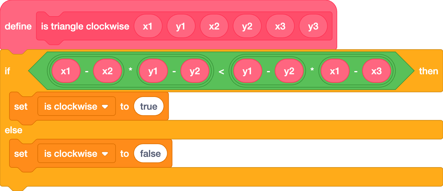
Normalize: sets a vector’s magnitude to 1, while retaining its direction.
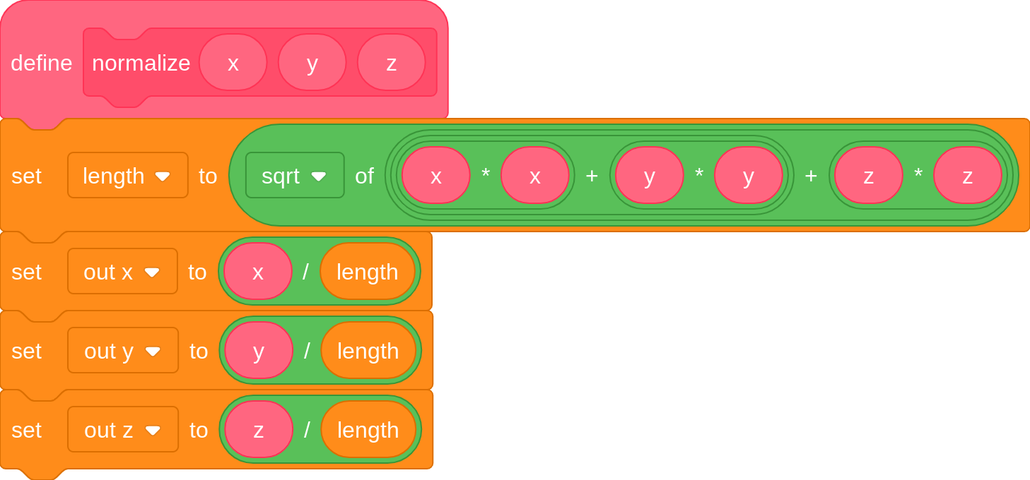
Transpose: Rotating the matrix format (For inverse TBN since inverse is expensive and they do the same thing in that case.)

Glossary
AABB :
Axis-Aligned Bounding Box (AABB) - A bounding box aligned with the axes of the coordinate system.
Buffer :
A section of memory used for temporary data storage.
BVH :
Bounding Volume Hierarchy (BVH) - A tree-based acceleration structure containing primitive 3D objects that speeds up ray-casting and various algorithms.
Camera Space :
(Also known as; View Space, Eye Space) - 3D coordinates projected relative to the camera, including relative depth.
Cross Product :
An operation between two vectors which returns a vector perpendicular to the two input vectors. The magnitude of this vector is the product of the magnitudes of the input vectors and the sine of the angle formed between the vectors.
Lerp :
Linear Interpolation.
Depth Buffer :
An additional screen-space buffer that provides depth information.
DOF :
Depth of Field (DOF) - The distance between the nearest and the furthest objects that are in acceptably sharp focus in an image captured with a camera.
Dot Product :
An operation between two vectors that returns the product of their magnitudes and the cosine of the angle between them.
Epsilon :
A very small value, mostly used to prevent floating-point inaccuracies and to set ray marching limits.
Focal Length :
A camera property that indicates how strongly it converges or diverges light. It is inversely proportional to the Field of View (FOV).
FOV :
Field of View (FOV) - The angular extent of the world that is seen. It is inversely proportional to the focal length.
Length :
The magnitude of a vector.
Magnitude :
The length of a vector.
Mesh :
A collection of faces, edges, and vertices that define an object's shape.
Model Space :
(Also known as; Object Space, Local Space) - 3D coordinates relative to another point of reference, typically used to store meshes of individual models or objects.
Surface Normal :
A vector perpendicular to the surface of an object.
Pen :
A vanilla Scratch extension used to draw on the screen.
Procedural :
Defined by code.
Rasterizer :
An algorithm that draws objects to the screen by filling in shapes pixel-by-pixel.
Ray :
Defined by its origin (a position in 3D space where the ray starts) and its direction.
Screen Space :
(Also known as; Clip Space) - 2D information of 3D coordinates projected to the screen, without depth information.
SDF :
Signed Distance Field (SDF) - A function defining distance to the surface of an object, with interior points being negative and exterior points being positive.
Vector :
An object having direction as well as magnitude, used to determine the position of one point in space relative to another.
Vertex :
A point with a coordinate vector.
Viewing Frustum :
The region of space in the modeled world that may appear on the screen.
World Space :
3D coordinates relative to the center of the world, typically (0, 0, 0).
Credits
Authors
- scratchtomv
- BamBozzle
- badatcode123
- Urlocalcreator
- insanetaco2000 (derpy gamer)
- Bigbrain123321
- TheGreenFlash
- jfs22
- littlebunny06
- 26243AJ
- KryptoScratcher (Krypto)
- SpinningCube
- Alltrue
- Meunspeakable
- Rinostar
- TheReal_BestGamer
- Robostew
Thanks
By the 3D Graphics and Scratch community. Thanks to littlebunny06 for the original idea, and jfs22 for launching the project on the 13th of June of 2024.
Screenshots taken from : scratch.mit.edu, wikipedia.org, iquilezles.org
Scratch code screenshots taken with scratchaddons.com
Front-page image : Factory Building [3D] by awesome-llama
Some illustrations of The Basics by scratchtomv
Made with mdbook.